Sum a row of values and redistribute the data in groups of 10.

[Gaztron3000]

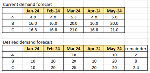
I am trying to forecast customer demand for a product. Using order history, i can estimate a customer's average monthly order, however, some values have decimal points and there is a minimum order quantity required.
I want to write a formula that adds up the total value across a row of data (estimated orders per month) and redistributes the data in groups of 10 (minimum order quantity) across the same number of cells.

example: see attached image.

Is it possible to set a different redistribution value for different customers based on known historical order quantities?

Thanks for any help you can give.

 

[Peter_SSs]

Welcome to the MrExcel board!

For the future I suggest that you investigate XL2BB for providing sample data to make it easier for helpers by not having to manually type out sample data to test with.

See if this does what you want

23 11 08.xlsm
	A	B	C	D	E	F	G
1
2	A	4	4	5	4	5
3	B	16	16	20	16	20
4	C	16.8	16.8	21	16.8	21
5
6
7	A			10		10	2
8	B	10	20	20	10	20	8
9	C	10	20	20	20	20	2.4
Demand

Cell Formulas
Range	Formula
B7:F9	B7	=LET(f,SUM($B2:B2),u,SUM($A7:A7),IF(f>u+10,INT((f-u)/10)*10,""))
G7:G9	G7	=SUM(B2:F2)-SUM(B7:F7)

 

[Gaztron3000]

Thank you, Peter. You are a genius.
This is my first time using the site, so my apologies for not using the XL2BB. I will be sure to use it next time.
Thanks for your help.

 

[Peter_SSs]

You're welcome, but I believe that there is an error with my formula (Missing an = sign)

See the example below. My original formula is in row 7 and what I think the corrected version should be in row 12.

23 11 08.xlsm
	A	B	C	D	E	F	G
2	A	10	6	4	10	10
6
7	A		10		20		10
11
12	A	10		10	10	10	0
Demand

Cell Formulas
Range	Formula
B7:F7	B7	=LET(f,SUM($B2:B2),u,SUM($A7:A7),IF(f>u+10,INT((f-u)/10)*10,""))
G7	G7	=SUM(B2:F2)-SUM(B7:F7)
B12:F12	B12	=LET(f,SUM($B2:B2),u,SUM($A12:A12),IF(f>=u+10,INT((f-u)/10)*10,""))
G12	G12	=SUM(B2:F2)-SUM(B12:F12)