Sum Across Multiple Columns with date Critieria Across the header

ChetanPuri

Board Regular
Joined
Sep 5, 2018
Messages
60
Office Version
  1. 365
Platform
  1. Windows
Good Afternoon Excel Team,

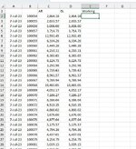
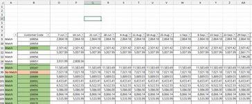
I need help with summing across Columns using both dates and Customer Code criteria. As you can see on Excel query Sheet 1, I have columns with Date Headers and underneath I have data, which I want to sum in sheet Column E, is there a formula where I can match the date and customer code in Column B of sheet 2 with Column B of Sheet 1 and it summs it by matching the header data and Colmn A dates in Sheet2. Any help with the formula is much appreciated.

Many thanks,

Regards,
Chetan
 

Attachments

  • Excel Query Sheet 2.jpg
    Excel Query Sheet 2.jpg
    119.1 KB · Views: 10
  • xecl Query Sheet 1.jpg
    xecl Query Sheet 1.jpg
    57.6 KB · Views: 9
Good news.

However, I don't see how Query 1 column E in your mini sheet is showing the results it is as the formula shown for that column is incorrect. :confused:
I think that part of the confusion with any checking that you have done is caused by the fact that you have so many identical values across a row in Query Sheet 2

=IFERROR(SUMIF('Query Sheet 2'!$A$2:$A$3000,'Query 1'!$B$2:$B$3000,INDEX('Query Sheet 2'!$B$2:$BA$123,0,MATCH('Query 1'!$A$2:$A$3000,'Query Sheet 2'!$1:$1,0)))," ")

SUMIF should have ranges that are the same size but those two red ranges are very different in size (number of rows).
Also your MATCH function is looking at the blue range so will find the column with the correct date. Suppose that match returns a '3' you would then be indexing column 3 of a range starting at column B (the second red one above). Column 3 of that red range is actually column 4 on the worksheet which would not be the column with the matching date.
An example of this with your data/formula is code 100074 for 7-Jul-23. Your results sheet shows 3490.98 but if you look at Query Sheet 2 for that code/date all the cells are blank meaning the result should be 0.

I would also highly recommend not using space characters for the IFERROR alternative and not using the sheet name that the formula is on (Query 1) within the formula as that can lead to incorrect results in some circumstances.

I believe that your formula for A2 should be this, copied down
=IFERROR(SUMIF('Query Sheet 2'!$A$2:$A$3000,B2,INDEX('Query Sheet 2'!$A$2:$BA$3000,0,MATCH(A2,'Query Sheet 2'!$1:$1,0))),"")
Initially I had the incorrect formula, but had fixed it since:
SIL Revenue Review 16 Feb 2024.xlsx
ABCDE
1DateCustomer CodeAR GLWorkSheet
27-Jul-231000542,864.182,864.182,864.18
37-Jul-231000552,633.572,633.572,501.42
47-Jul-231000565,008.005,008.005,007.99
57-Jul-231000573,714.733,714.733,931.99
67-Jul-2310005812,592.4512,592.4512,570.25
77-Jul-231000596,334.266,334.266,203.59
87-Jul-231000605,449.285,449.285,450.00
97-Jul-231000616,210.116,210.117,101.60
107-Jul-231000628,383.658,383.657,963.52
117-Jul-231000636,124.736,124.735,870.07
127-Jul-231000643,292.983,292.983,906.65
137-Jul-231000655,739.635,739.635,450.74
147-Jul-231000668,961.578,961.578,570.38
157-Jul-231000679,789.949,789.949,297.19
167-Jul-2310006810,483.0510,483.0510,604.93
177-Jul-231000694,052.174,052.174,894.06
187-Jul-231000707,186.277,186.276,771.87
197-Jul-231000718,386.048,386.047,965.81
207-Jul-231000726,510.356,510.356,510.34
217-Jul-231000734,860.024,860.024,860.02
227-Jul-231000743,676.003,676.000.00
237-Jul-231000754,877.044,877.044,631.57
247-Jul-231000765,175.575,175.575,175.57
257-Jul-231000774,794.364,794.364,794.35
267-Jul-231000784,437.014,437.014,188.60
277-Jul-231000796,254.796,254.796,660.95
287-Jul-231000815,039.155,039.154,728.55
297-Jul-231000824,210.714,210.714,210.71
307-Jul-231000834,226.164,226.164,216.41
317-Jul-2310008410,508.9610,508.969,980.02
327-Jul-231000855,369.245,369.245,098.99
337-Jul-231000866,751.666,751.666,411.83
347-Jul-231000876,675.196,675.196,657.27
357-Jul-231000880.007,393.307,021.18
367-Jul-231000895,889.035,889.035,889.03
377-Jul-231000916,638.446,638.446,433.41
387-Jul-231000926,868.256,868.256,522.55
397-Jul-231000935,014.395,014.395,086.00
407-Jul-231000946,172.336,172.338,866.14
417-Jul-231000954,878.324,878.324,632.78
427-Jul-231000965,230.495,230.494,926.75
437-Jul-231000984,408.474,408.474,186.58
447-Jul-231000996,562.376,562.376,232.08
457-Jul-2310010016,915.2916,915.2914,765.42
467-Jul-2310017214,297.3414,297.3413,577.72
477-Jul-231001859,803.549,803.549,310.10
487-Jul-231001945,792.535,792.535,500.98
497-Jul-231002294,136.614,136.614,632.87
507-Jul-2310023910,009.0310,009.0310,768.81
517-Jul-231002459,295.589,295.589,268.60
527-Jul-2310024612,020.3812,020.3811,415.37
537-Jul-2310024712,230.4712,230.4711,583.69
3 Way Rec
Cell Formulas
RangeFormula
C2:C53C2=SUMIFS(Data!$G:$G,Data!$B:$B,'3 Way Rec'!$B:$B,Data!$A:$A,">="&'3 Way Rec'!$A:$A,Data!$A:$A,"<="&'3 Way Rec'!$A:$A)
D2:D53D2=-SUMIFS(Revenue!$G:$G,Revenue!$J:$J,'3 Way Rec'!$B:$B,Revenue!$B:$B,">="&'3 Way Rec'!$A:$A,Revenue!$B:$B,"<="&'3 Way Rec'!$A:$A)
E2:E53E2=IFERROR(SUMIF('SIL July 2023-2024'!$B$9:$B$130,'3 Way Rec'!$B$2:$B$2249,INDEX('SIL July 2023-2024'!$O$9:$BN$130,0,MATCH('3 Way Rec'!$A$2:$A$2249,'SIL July 2023-2024'!$O$8:$BN$8,0))),"0")
Named Ranges
NameRefers ToCells
Data!ExternalData_1=Data!$A$1:$L$2602C2:C53
 
Upvote 0

Excel Facts

Wildcard in VLOOKUP
Use =VLOOKUP("Apple*" to find apple, Apple, or applesauce
That still looks wrong/risky to me

  • It still contains the worksheet name of the worksheet that it is on ('3 Way Rec'). As I stated before, that can lead to incorrect results in some circumstances and you wouldn't necessarily know what, if anything, was incorrect. There is no need for that name to be in the formula.

  • Your profile shows Excel 365 but are you actually using this workbook in 365?

  • In cell E2 your formula contains '3 way Rec'!$B$2:$B$2249 and '3 way Rec'!$A$2:$A$2249. Apart from the sheet names that shouldn't be there, why do you have those whole ranges there? Isn't the formula in E2 only looking at the code in B2 and the date in A2? Compare to my formula structure in post 10 and post 8 where I have just used B2 and A2.
 
Upvote 0
That still looks wrong/risky to me

  • It still contains the worksheet name of the worksheet that it is on ('3 Way Rec'). As I stated before, that can lead to incorrect results in some circumstances and you wouldn't necessarily know what, if anything, was incorrect. There is no need for that name to be in the formula.

  • Your profile shows Excel 365 but are you actually using this workbook in 365?

  • In cell E2 your formula contains '3 way Rec'!$B$2:$B$2249 and '3 way Rec'!$A$2:$A$2249. Apart from the sheet names that shouldn't be there, why do you have those whole ranges there? Isn't the formula in E2 only looking at the code in B2 and the date in A2? Compare to my formula structure in post 10 and post 8 where I have just used B2 and A2.
Thank you, I got it instead of giving it a range I should only refer to A2 & B2 as and when I add more data at the Bottom it shouldn't limit to the range?
 
Upvote 0

Forum statistics

Threads
1,215,076
Messages
6,122,983
Members
449,092
Latest member
Mr Hughes

We've detected that you are using an adblocker.

We have a great community of people providing Excel help here, but the hosting costs are enormous. You can help keep this site running by allowing ads on MrExcel.com.
Allow Ads at MrExcel

Which adblocker are you using?

Disable AdBlock

Follow these easy steps to disable AdBlock

1)Click on the icon in the browser’s toolbar.
2)Click on the icon in the browser’s toolbar.
2)Click on the "Pause on this site" option.
Go back

Disable AdBlock Plus

Follow these easy steps to disable AdBlock Plus

1)Click on the icon in the browser’s toolbar.
2)Click on the toggle to disable it for "mrexcel.com".
Go back

Disable uBlock Origin

Follow these easy steps to disable uBlock Origin

1)Click on the icon in the browser’s toolbar.
2)Click on the "Power" button.
3)Click on the "Refresh" button.
Go back

Disable uBlock

Follow these easy steps to disable uBlock

1)Click on the icon in the browser’s toolbar.
2)Click on the "Power" button.
3)Click on the "Refresh" button.
Go back
Back
Top