Sum Left based on Cell Color

alexm3430

New Member
Joined
Aug 27, 2015
Messages
47
Office Version
  1. 365
Platform
  1. Windows
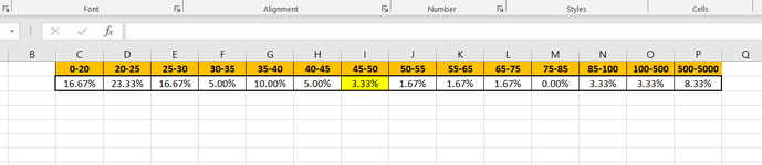
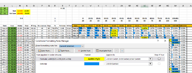
I have data in rows C2 thru P2. One of the cells is highlighted in yellow based on conditional formatting rule. The yellow cell is dynamic. For this exercise assume the yellow cell is I2. I want the formula to sum all cells to the left of I2 so cells C2 trhu H2 would be summed.
 

Attachments

  • Sum Left & Right.PNG
    Sum Left & Right.PNG
    16.8 KB · Views: 3

Excel Facts

What is the fastest way to copy a formula?
If A2:A50000 contain data. Enter a formula in B2. Select B2. Double-click the Fill Handle and Excel will shoot the formula down to B50000.
You can't use cell formatting to create a cell reference.

BUT,

You can use the Conditional Formatting rule you just mentioned. Please share that rule.

Additionally, please update your profile to show which version of excel you use. And, share your workbook as a mini worksheet using the xl2bb add in (link below). If you cannot use the add in, then post your data as a table.

Thanks in advance.
 
Last edited:
Upvote 0
You can't use cell formatting to create a cell reference.

BUT,

You can use the Conditional Formatting rule you just mentioned. Please share that rule.

Additionally, please update your profile to show which version of excel you use. And, share your workbook as a mini worksheet using the xl2bb add in (link below). If you cannot use the add in, then post your data as a table.

Thanks in advance.
abcdefghijklmnop
DateLive0-2020-2525-3030-3535-4040-4545-5050-5555-6565-7575-8585-100100-500500-5000
Feb-24$ 65.1516.67%23.33%16.67%5.00%10.00%5.00%3.33%1.67%1.67%1.67%0.00%3.33%3.33%8.33%
Mar-24$ 39.6014.49%17.39%24.64%14.49%7.25%4.35%4.35%4.35%5.80%0.00%1.45%1.45%0.00%0.00%
Apr-24$ 37.3811.11%15.87%15.87%9.52%4.76%1.59%7.94%7.94%12.70%4.76%3.17%3.17%1.59%0.00%
May-24$ 39.250.00%15.15%22.73%18.18%3.03%1.52%1.52%1.52%6.06%12.12%6.06%6.06%6.06%0.00%
Jun-24$ 59.300.00%1.52%9.09%19.70%9.09%6.06%6.06%3.03%0.00%4.55%12.12%12.12%15.15%1.52%
Jul-24$ 97.680.00%0.00%3.13%6.25%15.63%9.38%6.25%4.69%1.56%7.81%6.25%1.56%35.94%1.56%
Aug-24$ 152.080.00%0.00%0.00%1.47%2.94%10.29%5.88%4.41%2.94%5.88%5.88%11.76%41.18%7.35%
Sep-24$ 66.070.00%0.00%4.62%6.15%6.15%6.15%7.69%16.92%13.85%6.15%9.23%7.69%12.31%3.08%
Oct-24$ 38.641.56%6.25%4.69%4.69%9.38%10.94%7.81%9.38%21.88%10.94%3.13%3.13%4.69%0.00%
 
Upvote 0
What is the conditional formatting rule to define that cells turn yellow? I'm guessing in your example your threshold is 80%
 
Upvote 0
In your examples I do not see cells W5 or W6. Describing the rule in text as well may help. Are you unable to use xl2bb?

Also, your table post has columns A thru P, but your formatting applies to W thru AM, and W thru AI, how do you get column I to be yellow?

And what column do you want the sum of the queried range to be in?
 
Last edited:
Upvote 0
In your examples I do not see cells W5 or W6. Describing the rule in text as well may help. Are you unable to use xl2bb?

Also, your table post has columns A thru P, but your formatting applies to W thru AM, and W thru AI, how do you get column I to be yellow?

And what column do you want the sum of the queried range to be in?
Apologies for the confusion. I am unable to download XL2BB possibly because its my work desktop and it will not allow me. I attached an image that shows the work better.
 

Attachments

  • Sum Left Formula.PNG
    Sum Left Formula.PNG
    68.8 KB · Views: 7
Upvote 0
What happened to columns H and I? and everything to the left of I? Have you moved columns? What happened to the column labeled "Live"? How does the image here relate to your initial question?
Ive asked twice before... please provide a written description of what you want to occur? What numbers are being compared?

Forget the conditional formatting for a minute. Do you want to sum the cells in a row to the left a value that has met a certain condition. Which I'm guessing is when the sum of the cells from a fixed cell on the left to the current cell fall in between the two boundaries in rows 5 and 6?

Is that right?


And sending a table of the data in the picture would be a great help. I don't want to recreate you data from scratch.
I want the formula to find the cell highlighted in yellow. Then sum the values in columns V thru AC since cell AD is the one highlighted in yellow on the first row. The answer would be in cell AJ of the same row.
 
Upvote 0
i asked to ignore the conditional formatting and tell me what you want.
Plus, you've moved columns and rows around from the first table you posted.

SO, your conditional formatting is based on the value of "LIVE"

This is what I think the below worksheet does. NOTE: the column references are matched to the best of my abilitiy given your ambiguous details. My suggestion is to copy this into a fresh worksheet first to make sure you agree with the concept.

The concept is:
Step 1: Get one column before the column where the LIVE value is between the top and bottom values in rows 5 & 6 (if you haven't changed it).
Step 2: Start with the anchor column and sum until 1 column before the column identified in step 1.
Step 3 Sum those values.

This is using some functions in 365 that I am not super proficient with and I'm sure that some folks may come up with more elegant formulas. But, this works for the scenario I stated in the concept. If not, then PLEASE write out explicitly what you want, and provide a sample of data and expectations in a table and not an image.


Book1
UVWXYZAAABACADAEAFAGAHAIAJAKAL
1
2
3
4
5$0$20$25$30$35$40$45$50$55$65$75$85$100$500
6$20$25$30$35$40$45$50$55$65$75$85$100$500$5,000
7
8LiveDate0-2020-2525-3030-3535-4040-4545-5050-5555-6565-7575-8585-100100-500500-5000
9$65.152024-02-2416.67%23.33%16.67%5.00%10.00%5.00%3.33%1.67%1.67%1.67%0.00%3.33%3.33%8.33%83.34%
10$39.602024-03-2414.49%17.39%24.64%14.49%7.25%4.35%4.35%4.35%5.80%0.00%1.45%1.45%0.00%0.00%71.01%
11$37.382024-04-2411.11%15.87%15.87%9.52%4.76%1.59%7.94%7.94%12.70%4.76%3.17%3.17%1.59%0.00%52.37%
12$39.252024-05-240.00%15.15%22.73%18.18%3.03%1.52%1.52%1.52%6.06%12.12%6.06%6.06%6.06%0.00%56.06%
13$59.302024-06-240.00%1.52%9.09%19.70%9.09%6.06%6.06%3.03%0.00%4.55%12.12%12.12%15.15%1.52%54.55%
14$97.682024-07-240.00%0.00%3.13%6.25%15.63%9.38%6.25%4.69%1.56%7.81%6.25%1.56%35.94%1.56%60.95%
15$152.082024-08-240.00%0.00%0.00%1.47%2.94%10.29%5.88%4.41%2.94%5.88%5.88%11.76%41.18%7.35%51.45%
16$66.072024-09-240.00%0.00%4.62%6.15%6.15%6.15%7.69%16.92%13.85%6.15%9.23%7.69%12.31%3.08%61.53%
17$38.642024-10-241.56%6.25%4.69%4.69%9.38%10.94%7.81%9.38%21.88%10.94%3.13%3.13%4.69%0.00%17.19%
Sheet3
Cell Formulas
RangeFormula
AL9:AL17AL9=INDEX(LET(top,$W$6:$AJ$6,bot,$W$5:$AJ$5,rytd,LET(ytd,LET(r, $W9:$AJ9,acc,SCAN(0,r,LAMBDA(a,b,a+b)),acc),ytd),rytd),SUM(SEQUENCE(1,COLUMNS($W$8:$AJ$8))*((($U9>$W$5:$AJ$5)*($U9<=$W$6:$AJ$6))))-1)
 
Upvote 0

Forum statistics

Threads
1,215,106
Messages
6,123,122
Members
449,096
Latest member
provoking

We've detected that you are using an adblocker.

We have a great community of people providing Excel help here, but the hosting costs are enormous. You can help keep this site running by allowing ads on MrExcel.com.
Allow Ads at MrExcel

Which adblocker are you using?

Disable AdBlock

Follow these easy steps to disable AdBlock

1)Click on the icon in the browser’s toolbar.
2)Click on the icon in the browser’s toolbar.
2)Click on the "Pause on this site" option.
Go back

Disable AdBlock Plus

Follow these easy steps to disable AdBlock Plus

1)Click on the icon in the browser’s toolbar.
2)Click on the toggle to disable it for "mrexcel.com".
Go back

Disable uBlock Origin

Follow these easy steps to disable uBlock Origin

1)Click on the icon in the browser’s toolbar.
2)Click on the "Power" button.
3)Click on the "Refresh" button.
Go back

Disable uBlock

Follow these easy steps to disable uBlock

1)Click on the icon in the browser’s toolbar.
2)Click on the "Power" button.
3)Click on the "Refresh" button.
Go back
Back
Top