Sum/Merge only certain duplicates.

[wAtcHer1]

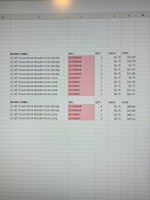
I apologize if I am not wording this correctly. I am new to this. I am hoping for a VBA that can solve this issue. Currently I am not using one. I normally find VBA’s online to use, I do not write them myself. The system we have at work is Microsoft 365 and we are still running Windows 10 Pro. I have a column/row with duplicate identifiers (SKU) and another column with pricing (EACH). I need to merge the duplicate identifiers that only have the same pricing and leave the duplicate with different pricing in place. My system will not let me download XL2BB so can only provide an image.

 

[alansidman]

I still would like to learn more about Power Query.

check out the Mr Excel Bookstore for a Book By Ken Puls and Miguel Escobar on Power Query

 

[wAtcHer1]

Thank you I will.

 

[kweaver]

Another way of looking at creating the uniques and then splitting them out per your sheet:

051923 Sum Spreadsheet.xlsm
	A	B	C	D	E
1	WORK FORMS	SKU	QTY	EACH	COST
2	15-24" Tinsel Work Wreath Form: Burlap	XX7504W4	2	$5.75	$11.50
3	15-24" Tinsel Work Wreath Form: Burlap	XX7504W4	2	$5.75	$11.50
4	15-24" Tinsel Work Wreath Form: Burlap	XX7504W4	1	$5.75	$5.75
5	15-24" Tinsel Work Wreath Form: Burlap	XX7504W4	3	$5.75	$17.25
6	15-24" Tinsel Work Wreath Form: Burlap	XX7504W4	4	$6.75	$27.00
7	15-24" Tinsel Work Wreath Form: Lime	XX750437	1	$5.75	$5.75
8	15-24" Tinsel Work Wreath Form: Lime	XX750437	2	$5.75	$11.50
9	15-24" Tinsel Work Wreath Form: Lime	XX750437	1	$5.75	$5.75
10	15-24" Tinsel Work Wreath Form: Lime	XX750437	3	$5.75	$17.25
11	15-24" Tinsel Work Wreath Form: Lime	XX750437	3	$6.75	$20.25
12
13
14		XX7504W4	5.75
15		XX7504W4	6.75
16		XX750437	5.75
17		XX750437	6.75
18
19		XX7504W4	8	5.75
20		XX7504W4	4	6.75
21		XX750437	7	5.75
22		XX750437	3	6.75
Sheet1

Cell Formulas
Range	Formula
E2:E11	E2	=C2*D2
B14:C17	B14	=UNIQUE(HSTACK(B2:B11,D2:D11))
B19:B22	B19	=FILTER(B14#,{1,0})
D19:D22	D19	=FILTER(B14#,{0,1})
C19:C22	C19	=SUMIFS($C$2:$C$11,$B$2:$B$11,$B19,$D$2:$D$11,$D19)
Dynamic array formulas.

 

[wAtcHer1]

Thank you for another option. I am currently using your first idea, but also trying to figure out the power query. I have a lot of worksheets with rows of this type of data. Figuring out which will be the best fit.

 

[wAtcHer1]

check out the Mr Excel Bookstore for a Book By Ken Puls and Miguel Escobar on Power Query

Thank you, I was able to figure out how to use the Power Query. It worked beautifully.