Sum with multiple row

trduy1908

New Member
Joined
Nov 29, 2023
Messages
7
Office Version
  1. 365
Platform
  1. Windows
Hi Everyone,

I have table with 4 column A, B, C, D:
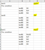
Data sample:

text A
Pre-condition
testB1OK
testB2N/Y
testB3NG
text B
testB1OK
testB2OK
testB3OK
testB4OK
testB5OK
text C
testB1OK
testB4N/Y
testB5OK

I want to fill value on column D with condition column D : ((C3:C5="False")+(C3:C5="N/Y"))>0,"False","Pass") on row D1, D6, D12 (D is dynamic) (value on D row base on value on column B or column C).
Please help me or suggest keyword to search.

Thanks a lot.

1705948014751.png
 

Excel Facts

Did you know Excel offers Filter by Selection?
Add the AutoFilter icon to the Quick Access Toolbar. Select a cell containing Apple, click AutoFilter, and you will get all rows with Apple
I think there are some ambiguous parts in your set up.
Can you explain what you're testing with the C3:C5="false" portion? I don't see any places in column C where the word "false" seems to be a value that would appear.

Also, what is the signifance of the "Pre-condition" row in Row 2?

As you can see below, breaking out your formula into to smaller calculations you get a mostly false results. Are you requiring all test for each text to be OK or NG, or at least one test in the text ranges?

Cell Formulas
RangeFormula
E3:E5,E13:E15,E7:E11E3=C3="False"
F3:F5,I13:I15,F13:F15,I7:I11,F7:F11,I3:I5F3=FORMULATEXT(E3)
H3:H5,H13:H15,H7:H11H3=C3="N/Y"
 
Upvote 0
Thanks! Your response awoohaw.

So all value in column A, B, C, I will be input data by hand, example: C3: OK, C4: False, C5: N/Y (I have list value {OK, False, N/A, NG} to input on column C)

Also, what is the signifance of the "Pre-condition" row in Row 2? -> "Pre-condition" is only text, and it's inputted by hand (it's occasionally or not)

I want to value on D (detail D1, D6 or D12 base on value on column example: D1 (C3: C5), D6 (C7:C11), D12 (C14:C18))

1706028977078.png

If the number of lines increases (or decreases) so D1 (C3:C7), D6 change to D8 ( C9: C13) and D12 change to D14 (C16:C20) (The value of the cell in Column C can change and input by hand)
1706029301367.png
 

Attachments

  • 1706028817293.png
    1706028817293.png
    17.2 KB · Views: 2
Upvote 0
I am pretty darn sure there is an easier way to do this. Power Query is a great tool, and I initially thought I could do that with only that.
But, as it turns out, my brain may not be thinking correctly, and I had to bring a table in from power query to use to do the final calculations.

So, the power query formula is this:

let
Source = Excel.CurrentWorkbook(){[Name="Table1"]}[Content],
#"Changed Type" = Table.TransformColumnTypes(Source,{{"Column1", type text}, {"Column2", type text}, {"Column3", type text}}),
#"Filtered Rows" = Table.SelectRows(#"Changed Type", each ([Column1] <> "Pre-condition")),
#"Filled Down" = Table.FillDown(#"Filtered Rows",{"Column1"}),
#"Filtered Rows1" = Table.SelectRows(#"Filled Down", each ([Column2] <> null))
in
#"Filtered Rows1"


And the worksheet is this:


Book1
ABCDEFGHIJKLMNO
1Column1Column2Column3OKColumn1Column2Column3
2text AFalsetext AtestB1OK
3Pre-conditionDataValidationListtext AtestB2N/Y
4testB1OKFalsetext AtestB3NG
5testB2N/YOKtext BtestB1OK
6testB3NGN/Ytext BtestB2OK
7text BPassNGtext BtestB3OK
8testB1OKtext BtestB4OK
9testB2OKtext BtestB5OK
10testB3OKtext CtestB1OK
11testB4OKtext CtestB4N/Y
12testB5OKtext CtestB5OK
13text CFalse
14testB1OK
15testB4N/Y
16testB5OK
17
Sheet7
Cell Formulas
RangeFormula
E2,E13,E7E2=IF(COUNTIFS(Table1_1[Column1],A2,Table1_1[Column3],"<>OK")<1,"Pass","False")
Cells with Data Validation
CellAllowCriteria
C4:C16List=$I$4:$I$7
 
Upvote 0
Solution

Forum statistics

Threads
1,215,139
Messages
6,123,263
Members
449,093
Latest member
Vincent Khandagale

We've detected that you are using an adblocker.

We have a great community of people providing Excel help here, but the hosting costs are enormous. You can help keep this site running by allowing ads on MrExcel.com.
Allow Ads at MrExcel

Which adblocker are you using?

Disable AdBlock

Follow these easy steps to disable AdBlock

1)Click on the icon in the browser’s toolbar.
2)Click on the icon in the browser’s toolbar.
2)Click on the "Pause on this site" option.
Go back

Disable AdBlock Plus

Follow these easy steps to disable AdBlock Plus

1)Click on the icon in the browser’s toolbar.
2)Click on the toggle to disable it for "mrexcel.com".
Go back

Disable uBlock Origin

Follow these easy steps to disable uBlock Origin

1)Click on the icon in the browser’s toolbar.
2)Click on the "Power" button.
3)Click on the "Refresh" button.
Go back

Disable uBlock

Follow these easy steps to disable uBlock

1)Click on the icon in the browser’s toolbar.
2)Click on the "Power" button.
3)Click on the "Refresh" button.
Go back
Back
Top