SumIF & Vlookup help

[Hobbit2010]

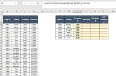
Hi can someone please help me with a formula to return value in the following blank columns highlighted in yellow in the example attached ?

In summary I want to pull currencies for each employee and a sum total of those currency in a separate column. In my analysis there are max two payment currencies for each employee.

Any speed injected in helping with the formula will be much appreciated.

Many thanks in advance.

 

[Coyotex3]

To start, in order to pull the currency you can do something like this:

TAKE(FILTER(C2:C9,(B2:B9=H2)*(A2:A9=G2)),1)

How do you want the currency displayed? Is there an order of preference? Shelly has USD and GBP. Which one would you like to pull? It is a bit hard to pull the data using a lookup since the table on the left does not contain unique values.

 

[Hobbit2010]

To start, in order to pull the currency you can do something like this:

TAKE(FILTER(C2:C9,(B2:B9=H2)*(A2:A9=G2)),1)

View attachment 107671

How do you want the currency displayed? Is there an order of preference? Shelly has USD and GBP. Which one would you like to pull? It is a bit hard to pull the data using a lookup since the table on the left does not contain unique values.

Thank you so much in looking into this, I am struggling to see what formula to use to return for example if we take Shelly I am after a formula which returns in cell I2 = USD; Cell J2=sum of USD (i.e $4000); cell K2 = GBP and then cell L2=6000 (i.e. sum of GBP amount. Do you think its possible via a combination of vlookup, IF and SumIF formula or any other way to return those values? Thank you so much in advance.

 

[Alex Blakenburg]

It is a bitty risky assuming 2 currencies.
This might work for your yellow columns.

Your are indicating you are using 2 versions of Excel. I am not sure that 2021 supports Take.

20240229 Extract and Sum 2 currencies Hobbit2010.xlsx
	A	B	C	D	E	F	G	H	I	J	K	L
1
2	Emp ID	Name	Currency	Amount			Emp ID	Name	Currency 1	Sum amt	Currency 2	sum amount 2
3	1001	Shelly	USD	1000			1001	Shelly	USD	4000	GBP	6000
4	1001	Shelly	GBP	2000			1002	Kim	AUD	18000	USD	8000
5	1001	Shelly	USD	3000
6	1001	Shelly	GBP	4000
7	1002	Kim	AUD	5000
8	1002	Kim	AUD	6000
9	1002	Kim	AUD	7000
10	1002	Kim	USD	8000
Sheet1

Cell Formulas
Range	Formula
I3:I4	I3	=XLOOKUP(G3,$A$3:$A$10,$C$3:$C$10,"")
J3:J4	J3	=SUMIFS($D$3:$D$10,$A$3:$A$10,$G3,$C$3:$C$10,I3)
K3:K4	K3	=XLOOKUP(1,($A$3:$A$10=G3)*($C$3:$C$10<>$I3),$C$3:$C$10,"")
L3:L4	L3	=IF(K3<>"",SUMIFS($D$3:$D$10,$A$3:$A$10,$G3,$C$3:$C$10,K3),"")

 

[kevin9999]

Similar approach to Alex.

Book1
	A	B	C	D	E	F	G	H	I	J	K
1
2	Emp ID	Name	Currency	Amount		Emp ID	Name	Currency 1	amount	Currency 2	amount
3	1001	Shelly	USD	1,000		1001	Shelly	USD	4,000	GBP	6,000
4	1001	Shelly	GBP	2,000		1002	Kim	AUD	5,000	GBP	30,000
5	1001	Shelly	USD	3,000		1003	Bridget	GBP	46,000	AUD	14,000
6	1001	Shelly	GBP	4,000		1004	Kyle	AUD	15,000
7	1002	Kim	AUD	5,000		1005	Andrew	USD	16,000	AUD	17,000
8	1002	Kim	GBP	6,000		1006	Tim	AUD	18,000	GBP	39,000
9	1002	Kim	GBP	7,000
10	1002	Kim	GBP	8,000
11	1002	Kim	GBP	9,000
12	1003	Bridget	GBP	10,000
13	1003	Bridget	GBP	11,000
14	1003	Bridget	GBP	12,000
15	1003	Bridget	GBP	13,000
16	1003	Bridget	AUD	14,000
17	1004	Kyle	AUD	15,000
18	1005	Andrew	USD	16,000
19	1005	Andrew	AUD	17,000
20	1006	Tim	AUD	18,000
21	1006	Tim	GBP	19,000
22	1006	Tim	GBP	20,000
23
Sheet2

Cell Formulas
Range	Formula
G3:G8	G3	=VLOOKUP(F3,$A$3:$B$22,2,FALSE)
H3:H8	H3	=VLOOKUP(F3,$A$3:$C$22,3,FALSE)
I3:I8	I3	=SUMIFS($D$3:$D$22,$A$3:$A$22,$F3,$C$3:$C$22,H3)
J3:J8	J3	=UNIQUE(FILTER($C$3:$C$22,($A$3:$A$22=F3)*($C$3:$C$22<>H3),""))
K3:K8	K3	=IF(J3<>"",SUMIFS($D$3:$D$22,$A$3:$A$22,$F3,$C$3:$C$22,J3),"")

 

[Hobbit2010]

Thank you Alex and Kevin, can I please check if the two tables are in separate tabs if the above formulas should work, cause as soon as I am pulling the same columns as suggested by you from a different tab for SUMIFS formula it is giving me an error of too many arguments put in. For clarity I have column A to D in Tab 2 and Tab 1 has the highlighted cells where I want to input the formula. I am new to this forum so not sure how to upload the worksheet for ease. I am using microsoft 365 excel version for my analysis. Thank you again.

 

[kevin9999]

Shouldn't be a problem:

Book1
	A	B	C	D	E
1
2	Emp ID	Name	Currency	Amount
3	1001	Shelly	USD	1,000
4	1001	Shelly	GBP	2,000
5	1001	Shelly	USD	3,000
6	1001	Shelly	GBP	4,000
7	1002	Kim	AUD	5,000
8	1002	Kim	GBP	6,000
9	1002	Kim	GBP	7,000
10	1002	Kim	GBP	8,000
11	1002	Kim	GBP	9,000
12	1003	Bridget	GBP	10,000
13	1003	Bridget	GBP	11,000
14	1003	Bridget	GBP	12,000
15	1003	Bridget	GBP	13,000
16	1003	Bridget	AUD	14,000
17	1004	Kyle	AUD	15,000
18	1005	Andrew	USD	16,000
19	1005	Andrew	AUD	17,000
20	1006	Tim	AUD	18,000
21	1006	Tim	GBP	19,000
22	1006	Tim	GBP	20,000
23
Tab 2

Book1
	A	B	C	D	E	F
1	Emp ID	Name	Currency 1	amount	Currency 2	amount
2	1001	Shelly	USD	4,000	GBP	6,000
3	1002	Kim	AUD	5,000	GBP	30,000
4	1003	Bridget	GBP	46,000	AUD	14,000
5	1004	Kyle	AUD	15,000
6	1005	Andrew	USD	16,000	AUD	17,000
7	1006	Tim	AUD	18,000	GBP	39,000
8
Tab 1

Cell Formulas
Range	Formula
B2:B7	B2	=VLOOKUP(A2,'Tab 2'!$A$3:$B$22,2,FALSE)
C2:C7	C2	=VLOOKUP(A2,'Tab 2'!$A$3:$C$22,3,FALSE)
D2:D7	D2	=SUMIFS('Tab 2'!$D$3:$D$22,'Tab 2'!$A$3:$A$22,$A2,'Tab 2'!$C$3:$C$22,C2)
E2:E7	E2	=UNIQUE(FILTER('Tab 2'!$C$3:$C$22,('Tab 2'!$A$3:$A$22=A2)*('Tab 2'!$C$3:$C$22<>C2),""))
F2:F7	F2	=IF(E2<>"",SUMIFS('Tab 2'!$D$3:$D$22,'Tab 2'!$A$3:$A$22,$A2,'Tab 2'!$C$3:$C$22,E2),"")

 

[kevin9999]

To upload a worksheet, you could download the XL2BB add in, or alternatively, share your file via Google Drive, Dropbox or similar file sharing platform - just remember to make the file available to anyone with the link

 

[Hobbit2010]

Thank you heaps Kevin, this has saved so much of my time and energy . Really appreciate all the help and so glad I joined this forum .

 

[kevin9999]

Glad we were able to help & welcome to the Forum.
Given that you have 365, it would be worth learning about the XLOOKUP functions that @Alex Blakenburg suggested in post #4