Sumifs array question

[cuddy89]

I would be very grateful for assistance with the following query which I have spent a while trying to figure out (on a Sunday!)

Please see the attached spreadsheet which contains some sample data.

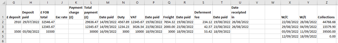
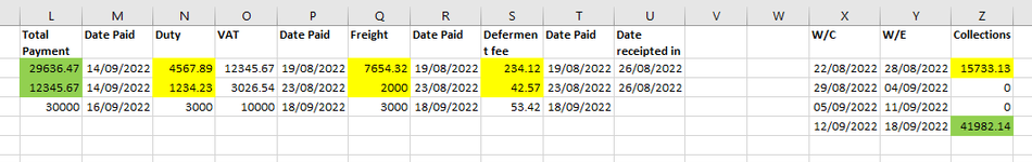
In column Z, I require columns G,L,N and Q to be summed based on the date to their right, so H,M,P and R.

This is conditional on the below:

There being a date in column U (so non-blank).

The date in column U being greater or equal to the date in column X

The dates in H,M,P and R need to be less than or equal to the date in column Y

Where I am coming unstuck is when column U's date is earlier than the date in any of H,M,P and R

For example, for row 2, £15,366.33 would be the value given in cell Z2, but then £29,636.47 would be given in cell Z5 for row 2.

I think I need to write a sumifs formula in an array for this, but I am struggling to work out how to write this.

Thanks in advance.

Richard

 

[RoryA]

So you're saying that 15,366.33 should not be the answer in Z2?

 

[cuddy89]

So you're saying that 15,366.33 should not be the answer in Z2?

No, it shouldnt.

I have attached a picture highlighting which values go in which Z cell (and removed deposits just to keep it simple, my problem remains the same).

The formula in Z needs to work as follows:

When there is a date in U, any of L,N,Q and S which have a corresponding date to the right (M,P,R,T) which is less than or equal to U, are summed if U falls between the values in X and Y

The 2 cells highlighted green (L2,L3) are summed in Z5 as their date in column M is after the date in column U, so need to be summed between the correct X and Y values.

I hope that makes sense.

 

[RoryA]

We seem to have changed columns now too. Can you move column N next to P, since it's the only one that is not dependent on the column immediately to the right, and that throws any pattern out.

 

[cuddy89]

Sorry Rory, too many spreadsheets open!

To confirm, only L, N and Q.

You can delete out column O on Alex's XL2BB sheet if you like as it isnt needed to write the formula.

 

[RoryA]

But is it actually there in your real sheet? It should be a relatively straightforward SUMPRODUCT formula if each value column is immediately to the left of the relevant date column, but in your picture that one is not - it's two columns to the left. That will make it much harder to write a simple formula.

 

[cuddy89]

Yes it is there in my real sheet, but if you need me to move columns around in order for you to be able to solve my query then I can do.

 

[RoryA]

If you can move it, then I think this would work:

=SUMPRODUCT(($U$2:$U$4>=X2)*($M$1:$T$1="Date Paid")*($M$2:$T$4<=Y2)*$L$2:$S$4)

adjust the row numbers as needed.

 

[cuddy89]

Thanks Roy

I have tried using this but it doesn't seem to account for when the date paid is greater than the date receipted in.

So the payments in L2 and L3 are not being summed in Z5 (as on the attached picture).

I think this is because the first part of the formula - SUMPRODUCT(($U$2:$U$4>=X2) will not return a value for Z5

Please can you let me know if you have a solution to this.

 

[RoryA]

Per your requirements:

When there is a date in U, any of L,N,Q and S which have a corresponding date to the right (M,P,R,T) which is less than or equal to U, are summed if U falls between the values in X and Y

 

[cuddy89]

Sorry Roy, they also need to be summed if U is less than or equal to the values between X and Y, but the date in M,P,R,T falls between the values in X and Y