Sumifs Formula

[SJC27x5]

Please help in fixing this issue with sumifs

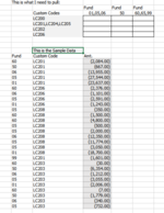
Cell A1 to A100 has serial numbers 1 to 100, Cell B1 to B100 has corresponding sales values. I am trying to the get the total of values based on the criteria 45,55,65

Sumifs(B1:B100,A1:A100,criteria 1)

Here criteria 1 has to be 45, 55, 65

I hope you are able the understand the requirement, please help.. I need sumifs itself, since I have other criteria range and criteria which is unique.

Thank you.

 

[Eric W]

Welcome to the forum!

Is this what you want?

Book1 (version 1).xlsb
	A	B	C	D	E	F
1	1	1		Sum	Sum	List
2	2	2		71	71	45
3	3	3				55
4	45	4				65
5	6	5
6	7	6
7	55	7
8	6	8
9	55	9
10	55	10
11	4	11
12	45	12
13	45	13
14	77	14
15	88	15
16	65	16
17	1	17
18	2	18
19	3	19
20	4	20
Sheet24

Cell Formulas
Range	Formula
D2	D2	=SUM(SUMIFS(B1:B20,A1:A20,{45,55,65}))
E2	E2	=SUM(SUMIFS(B1:B20,A1:A20,F2:F4))

 

[jtakw]

Hi,

Try this:

Book3.xlsx
	A	B	C	D
1	43	2		47
2	44	3
3	45	4
4	46	5
5	47	6
6	43	7
7	54	8
8	55	9
9	56	10
10	47	11
11	43	12
12	44	13
13	64	14
14	65	15
15	66	16
16	43	17
17	44	18
18	45	19
19	46	20
20	47	21
Sheet898

Cell Formulas
Range	Formula
D1	D1	=SUM(SUMIFS(B1:B100,A1:A100,{45,55,65}))

 

[SJC27x5]

Welcome to the forum!

Is this what you want?

Book1 (version 1).xlsb
	A	B	C	D	E	F
1	1	1		Sum	Sum	List
2	2	2		71	71	45
3	3	3				55
4	45	4				65
5	6	5
6	7	6
7	55	7
8	6	8
9	55	9
10	55	10
11	4	11
12	45	12
13	45	13
14	77	14
15	88	15
16	65	16
17	1	17
18	2	18
19	3	19
20	4	20
Sheet24

Cell Formulas
Range	Formula
D2	D2	=SUM(SUMIFS(B1:B20,A1:A20,{45,55,65}))
E2	E2	=SUM(SUMIFS(B1:B20,A1:A20,F2:F4))

Yes, D2, works fine..

Thank you...

 

[Eric W]

Glad we could help! Thanks for the feedback.

 

[cwbasset]

I'm hoping you can help with a very complex problem.

I need a sumifs formula that can match multiple criteria options in a range. I would really like to use cell references if possible as some of the criteria options will change in the future.

Example:

Sum_range:

Range 1: "Fund Codes" - Criteria 1: ""50"}; Criteria 2: {"60","65", "99"} Criteria 3: {"01", "05","06","17","20"} etc.

Range 1: "Fund Codes" - Criteria 1: ""OE150"}; Criteria 2: {"OR310", "OR311", "OR350"} etc.

 

[jtakw]

Hi,

You listed your 2 different requirement separately.
Are you looking for 1 formula or 2?

Your requirements Only show 1 Range ("Fund Codes"), I assume that's the Criteria Range, where's the Sum Range?
Please clarify all and may be a bit more explanation.

 

[cwbasset]

Sorry for the confusion. My question posted before I was ready and I wasn't sure how to edit it. Anyways, I have included an image of a small part of what I need to pull out of the raw data. Each column is for a fund code, and it could be only one code, or a combination of up to seven funds combined into one column. Each line is for custom codes. Again, The line could be for only one custom code, or up to six. I have used =sum(sumifs(...)) formulas in the past, but when we get to the maximum combinations of funds and custom codes, it just wouldn't work.

Hope this clarifies the problem.

 

[jtakw]

Ok, thanks for clarifying.

If you want to use a more "Traditional" SUM/SUMIFS, you'll have to Separate out the "Custom Codes" in C4:C7, and the "Fund Codes" in D3:F3 into their Own individual cells.

Also, please check my signature to look into how to post sample data using XL2BB, so we don't have to re-type your data manually for testing, thanks.

Otherwise, this is one way we could do this:

Book3.xlsx
	A	B	C	D	E	F
1
2				Fund Codes
3			Custom Codes	01,05,06	50	60,65,99
4			LC200	0	0	0
5			LC201,LC204,LC205	15	3	22
6			LC202	0	0	0
7			LC206	27	0	7
8
9
10
11		Fund	Custom Codes
12		60	LC201	2
13		50	LC201	3
14		06	LC201	4
15		05	LC201	5
16		01	LC201	6
17		60	LC206	7
18		06	LC206	8
19		05	LC206	9
20		01	LC206	10
21		05	LC208	11
22		60	LC208	12
23		60	LC208	13
24		05	LC208	14
25		05	LC208	15
26		06	LC208	16
27		05	LC208	17
28		05	LC208	18
29		01	LC208	19
30		99	LC201	20
31		60	LC203	21
32		50	LC203	22
33		06	LC203	23
34		05	LC203	24
35		01	LC203	25
36		60	LC203	26
37		50	LC203	27
38		06	LC203	28
39		05	LC203	29
40
Sheet897

Cell Formulas
Range	Formula
D4:F7	D4	=SUMPRODUCT((ISNUMBER(SEARCH($C$12:$C$39,$C4))*ISNUMBER(SEARCH($B$12:$B$39,D$3)))*$D$12:$D$39)

 

[cwbasset]

Thank you so much for taking the time to help with this. I think we are getting closer, however, I must still be missing something. My data sheet is actually pretty large, so I am using named ranges. When I plug in this formula: =SUMPRODUCT((ISNUMBER(SEARCH(TB_Custom,$A13))*ISNUMBER(SEARCH(TB_Fund,D$80)))*TB_Round) I am getting a #VALUE! result.

Also, as I am using my work computer, I can't add the extension. Sorry!