Summarize using VBA Scripting Dictionary

[deba2020]

I have a data which contains 18 columns, I need to summarize the data based on the 1st 2 columns and in the summary there will be just 3 columns as shown in below table
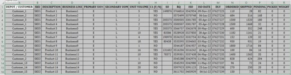
Raw Data in Sheet1

DEPOT / CUSTOMER	SKU	DESCRIPTION	BUSINESS LINE	PRIMARY UOM	SECONDARY UOM	UNIT VOLUME	C1 (Y/N)	SO	RQ	ISO	ISO DATE	DLV	ORDERED	SHIPPED	PENDING	PICKED	WEIGHT
Customer_1	SKU1	Product 1	Business1	E	L	5	YES	149876	3764816	3542954	09-Nov-22	37627225	110	28	82	0	0
Customer_2	SKU2	Product 2	Business2	E	L	1	NO		3575499	3370748	06-Jun-22	37627226	684	516	168	0	0
Customer_3	SKU1	Product 3	Business3	E	L	2	YES	205575	3500505	3301785	05-Apr-22	37627227	1500	1320	180	0	0
Customer_1	SKU1	Product 4	Business4	E	L	2	YES	205575	3500507	3301787	05-Apr-22	37627228	1500	1468	32	0	0
Customer_5	SKU5	Product 5	Business5	E	L	2	YES	205575	3566757	3362678	30-May-22	37627229	600	352	248	0	0
Customer_3	SKU1	Product 6	Business6	E	L	10	YES	83586	3528928	3327850	28-Apr-22	37627230	1182	1161	21	0	0
Customer_1	SKU1	Product 7	Business7	E	L	4	YES	190970	3534232	3332754	02-May-22	37627231	152	120	32	0	0
Customer_2	SKU1	Product 8	Business8	E	L	18	YES	80458	3535595	3334065	03-May-22	37627232	950	931	19	0	0
Customer_3	SKU2	Product 9	Business9	E	L	1	NO		3544187	3341957	10-May-22	37627233	1800	1716	84	0	0
Customer_1	SKU2	Product 10	Business10	E	L	16	YES	131602	3516206	3316242	18-Apr-22	37627234	100	84	16	0	0
Customer_2	SKU2	Product 11	Business11	E	L	10	YES	78372	3539301	3337438	06-May-22	37627235	1400	1365	35	0	0
Customer_2	SKU2	Product 12	Business12	E	L	1	NO		3545288	3342976	11-May-22	37627236	828	624	204	0	0
Customer_13	SKU2	Product 13	Business13	E	L	10	NO		3545293	3342980	11-May-22	37627237	96	72	24	0	0
Customer_14	SKU3	Product 14	Business14	E	L	20	NO		3597923	3391123	25-Jun-22	37627238	270	250	20	0	0
Customer_15	SKU2	Product 15	Business15	E	L	14	NO		3611702	3403929	06-Jul-22	37627239	150	71	79	0	0

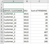
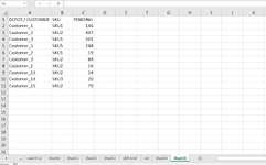
Need Summary in Sheet 2 as follows with these 3 columns (1st 2 columns and Sum of Column "Pending")

DEPOT / CUSTOMER	SKU	PENDING
Customer_1	SKU1	146
Customer_1	SKU2	16
Customer_13	SKU2	24
Customer_14	SKU3	20
Customer_15	SKU2	79
Customer_2	SKU1	19
Customer_2	SKU2	407
Customer_3	SKU1	201
Customer_3	SKU2	84
Customer_5	SKU5	248

 

[shinigamilight]

You can give this a try

Sub deba2020()
            Dim wk1 As Worksheet, wk2 As Worksheet
            Set wk1 = Sheets("sheet14")            ' change your input sheet
            Set wk2 = Sheets("sheet15")             'change your output sheet
            Dim lr, k As Long
            Dim V, S
           
            lr = wk1.Range("A" & Rows.Count).End(xlUp).Row
            Dim dic As Object
            Set dic = CreateObject("Scripting.Dictionary")
            Dim TempStore As String
            With wk1
                    For k = 2 To lr
                            TempStore = .Range("A" & k).Value & "|" & .Range("B" & k).Value
                            If dic.Exists(TempStore) = False Then
                                    dic(TempStore) = .Range("P" & k).Value
                            Else: dic(TempStore) = dic(TempStore) + .Range("P" & k).Value
                            End If
                    Next k
            End With
            k = 0
           

            With wk2
                For Each S In dic.Keys
                     V = Split(S, "|")
                     .Range("A" & Rows.Count).End(xlUp).Offset(1, 0).Resize(1, 2) = V
                Next S
                .Range("C" & Rows.Count).End(xlUp).Offset(1, 0).Resize(dic.Count) = WorksheetFunction.Transpose(dic.Items)
            End With
           
            S = Array("DEPOT / CUSTOMER", "SKU", "PENDING")
            wk2.Range("A1").Resize(1, UBound(S) + 1) = S
End Sub

 

[Peter_SSs]

What about using Excel's built-in Pivot Table feature (on the Insert ribbon tab)?

23 01 28.xlsm
	A	B														P			S	T	U	V	W
1	DEPOT / CUSTOMER	SKU														PENDING				DEPOT / CUSTOMER	SKU	Sum of PENDING
2	Customer_1	SKU1														82				Customer_1	SKU1	146
3	Customer_2	SKU2														168				Customer_1	SKU2	16
4	Customer_3	SKU1														180				Customer_13	SKU2	24
5	Customer_1	SKU1														32				Customer_14	SKU3	20
6	Customer_5	SKU5														248				Customer_15	SKU2	79
7	Customer_3	SKU1														21				Customer_2	SKU1	19
8	Customer_1	SKU1														32				Customer_2	SKU2	407
9	Customer_2	SKU1														19				Customer_3	SKU1	201
10	Customer_3	SKU2														84				Customer_3	SKU2	84
11	Customer_1	SKU2														16				Customer_5	SKU5	248
12	Customer_2	SKU2														35
13	Customer_2	SKU2														204
14	Customer_13	SKU2														24
15	Customer_14	SKU3														20
16	Customer_15	SKU2														79
Summary

 

[deba2020]

You can give this a try

Sub deba2020()
            Dim wk1 As Worksheet, wk2 As Worksheet
            Set wk1 = Sheets("sheet14")            ' change your input sheet
            Set wk2 = Sheets("sheet15")             'change your output sheet
            Dim lr, k As Long
            Dim V, S
          
            lr = wk1.Range("A" & Rows.Count).End(xlUp).Row
            Dim dic As Object
            Set dic = CreateObject("Scripting.Dictionary")
            Dim TempStore As String
            With wk1
                    For k = 2 To lr
                            TempStore = .Range("A" & k).Value & "|" & .Range("B" & k).Value
                            If dic.Exists(TempStore) = False Then
                                    dic(TempStore) = .Range("P" & k).Value
                            Else: dic(TempStore) = dic(TempStore) + .Range("P" & k).Value
                            End If
                    Next k
            End With
            k = 0
          

            With wk2
                For Each S In dic.Keys
                     V = Split(S, "|")
                     .Range("A" & Rows.Count).End(xlUp).Offset(1, 0).Resize(1, 2) = V
                Next S
                .Range("C" & Rows.Count).End(xlUp).Offset(1, 0).Resize(dic.Count) = WorksheetFunction.Transpose(dic.Items)
            End With
          
            S = Array("DEPOT / CUSTOMER", "SKU", "PENDING")
            wk2.Range("A1").Resize(1, UBound(S) + 1) = S
End Sub

Thank you very much. It worked exactly as I wanted!!

 

[deba2020]

What about using Excel's built-in Pivot Table feature (on the Insert ribbon tab)?

23 01 28.xlsm
	A	B														P			S	T	U	V	W
1	DEPOT / CUSTOMER	SKU														PENDING				DEPOT / CUSTOMER	SKU	Sum of PENDING
2	Customer_1	SKU1														82				Customer_1	SKU1	146
3	Customer_2	SKU2														168				Customer_1	SKU2	16
4	Customer_3	SKU1														180				Customer_13	SKU2	24
5	Customer_1	SKU1														32				Customer_14	SKU3	20
6	Customer_5	SKU5														248				Customer_15	SKU2	79
7	Customer_3	SKU1														21				Customer_2	SKU1	19
8	Customer_1	SKU1														32				Customer_2	SKU2	407
9	Customer_2	SKU1														19				Customer_3	SKU1	201
10	Customer_3	SKU2														84				Customer_3	SKU2	84
11	Customer_1	SKU2														16				Customer_5	SKU5	248
12	Customer_2	SKU2														35
13	Customer_2	SKU2														204
14	Customer_13	SKU2														24
15	Customer_14	SKU3														20
16	Customer_15	SKU2														79
Summary

I wrote some VBA code which runs before this consolidation so I wanted to eliminate manual consolidation using pivot table and to have the summary being prepared using scripting dictionary.

 

[Peter_SSs]

I wrote some VBA code which runs before this consolidation so I wanted to eliminate manual consolidation using pivot table and to have the summary being prepared using scripting dictionary.

Fair enough. This would be my method.

Sub Make_Summary()
  Dim d As Object
  Dim a As Variant
  Dim i As Long
  
  Set d = CreateObject("Scripting.Dictionary")
  With Sheets("Data").Range("A1").CurrentRegion '<- Edit sheet name to suit
    a = Application.Index(.Cells, Evaluate("row(1:" & .Rows.Count & ")"), Array(1, 2, 16))
  End With
  For i = 2 To UBound(a)
    d(a(i, 1) & ";" & a(i, 2)) = d(a(i, 1) & ";" & a(i, 2)) + a(i, 3)
  Next i
  With Sheets.Add(After:=Sheets(Sheets.Count))
    With .Range("A2:B2").Resize(d.Count)
      .Value = Application.Transpose(Array(d.Keys, d.Items))
      .Sort Key1:=.Columns(1), Order1:=xlAscending, Header:=xlNo
      .Columns(2).Insert
      .Columns(1).TextToColumns DataType:=xlDelimited, Semicolon:=True, Other:=False
      .Rows(0).Value = Application.Index(a, 1, 0)
      .EntireColumn.AutoFit
    End With
  End With
End Sub

 

[deba2020]

Fair enough. This would be my method.

Sub Make_Summary()
  Dim d As Object
  Dim a As Variant
  Dim i As Long
 
  Set d = CreateObject("Scripting.Dictionary")
  With Sheets("Data").Range("A1").CurrentRegion '<- Edit sheet name to suit
    a = Application.Index(.Cells, Evaluate("row(1:" & .Rows.Count & ")"), Array(1, 2, 16))
  End With
  For i = 2 To UBound(a)
    d(a(i, 1) & ";" & a(i, 2)) = d(a(i, 1) & ";" & a(i, 2)) + a(i, 3)
  Next i
  With Sheets.Add(After:=Sheets(Sheets.Count))
    With .Range("A2:B2").Resize(d.Count)
      .Value = Application.Transpose(Array(d.Keys, d.Items))
      .Sort Key1:=.Columns(1), Order1:=xlAscending, Header:=xlNo
      .Columns(2).Insert
      .Columns(1).TextToColumns DataType:=xlDelimited, Semicolon:=True, Other:=False
      .Rows(0).Value = Application.Index(a, 1, 0)
      .EntireColumn.AutoFit
    End With
  End With
End Sub

It worked fantastically...Summed up the data exactly as I wanted. Thanks.

 

[Peter_SSs]

You're welcome. Glad to offer options. Thanks for the follow-up.

Speaking of options, here is another fairly compact code, that does not require the dictionary object, that you could try.
Check the original data sheet name in the code still.

Sub Make_Summary_v2()
  Application.ScreenUpdating = False
  Sheets("Data").Copy After:=Sheets(Sheets.Count)
  With Sheets(Sheets.Count).UsedRange
    .Columns(3).FormulaR1C1 = Replace("=SUMIFS(R2C16:R#C16,R2C1:R#C1,RC1,R2C2:R#C2,RC2)", "#", .Rows.Count)
    .Columns(3).Value = .Columns(3).Value
    .Range("P1").Copy Destination:=.Range("C1")
    .Offset(, 3).Clear
    .Sort Key1:=.Columns(1), Order1:=xlAscending, Key2:=.Columns(2), Order2:=xlAscending, Header:=xlYes
    .RemoveDuplicates Columns:=Array(1, 2)
    .Columns.AutoFit
  End With
  Application.ScreenUpdating = True
End Sub

 

[deba2020]

You're welcome. Glad to offer options. Thanks for the follow-up.

Speaking of options, here is another fairly compact code, that does not require the dictionary object, that you could try.
Check the original data sheet name in the code still.

Sub Make_Summary_v2()
  Application.ScreenUpdating = False
  Sheets("Data").Copy After:=Sheets(Sheets.Count)
  With Sheets(Sheets.Count).UsedRange
    .Columns(3).FormulaR1C1 = Replace("=SUMIFS(R2C16:R#C16,R2C1:R#C1,RC1,R2C2:R#C2,RC2)", "#", .Rows.Count)
    .Columns(3).Value = .Columns(3).Value
    .Range("P1").Copy Destination:=.Range("C1")
    .Offset(, 3).Clear
    .Sort Key1:=.Columns(1), Order1:=xlAscending, Key2:=.Columns(2), Order2:=xlAscending, Header:=xlYes
    .RemoveDuplicates Columns:=Array(1, 2)
    .Columns.AutoFit
  End With
  Application.ScreenUpdating = True
End Sub

Humbled by the knowledge you possess. Both the solutions work perfectly. Thank you.

 

[Peter_SSs]

Cheers.