SUMPRODUCT and OFFSET

[Nanaia]

I have two formulas that you folks were kind enough to help me with that have thrown me a curve ball. They are supposed to provide a total for the month and the total for the year but are not showing the same result.

The value in A3 is 1.

Formula for the number of days that have a value in column NJ:

=SUMPRODUCT((OFFSET($A9,0,31*($A$3-1)+1,1,31)<>"")*(IF(OFFSET($A9,0,31*($A$3-1)+1,1,31)=$NR$16,0.5,IF(OFFSET($A9,0,31*($A$3-1)+1,1,31)=$NR$17,0.5,1))*(OFFSET($A$4,0,31*($A$3-1)+1,1,31))))

Formula for the number of days this year that have a value in column NK:

=SUMPRODUCT((OFFSET($A9,0,1,1,372)<>"")*(IF(OFFSET($A9,0,1,1,372)=$NR$16,0.5,IF(OFFSET($A9,0,1,1,372)=$NR$17,0.5,1))*(OFFSET($A$3,0,1,1,372))))

The data entered is only for the month of January so both results should be the same but they aren't. I am not very familiar with OFFSET so I am not sure how to resolve this issue. Can anyone help?

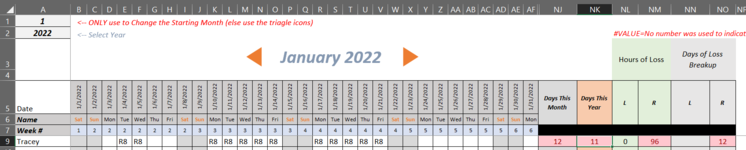
Attached is a screen shot of the results. Columns NJ and NK should show the same value but do not.

I cannot use XL2BB on this computer.

Thank you for your patience - and any help!

 

[StephenCrump]

Did this Forum provide these formulae? They imply you're allowing 31 columns for each month, and hence 372 days for the year, which must make your date formulae a little awkward? It would also be better not to use OFFSET() at all, as it's a volatile function.

The last term in the monthly formula, i.e. OFFSET($A$4,0,31*($A$3-1)+1,1,31) returns the range B4:AF4. This shows as blank in your screenshot, but must have numbers there (in white font?) otherwise your formula would return 0.

The last term in the yearly formula, OFFSET($A$3,0,1,1,372) will return a range in row 3, i.e. a different set of numbers (white font?) My first guess (it's impossible to tell from just a screenshot) is that this is causing the mismatch.

What's in the cells NR16 and NR17?

 

[Nanaia]

Did this Forum provide these formulae? They imply you're allowing 31 columns for each month, and hence 372 days for the year, which must make your date formulae a little awkward? It would also be better not to use OFFSET() at all, as it's a volatile function.

The last term in the monthly formula, i.e. OFFSET($A$4,0,31*($A$3-1)+1,1,31) returns the range B4:AF4. This shows as blank in your screenshot, but must have numbers there (in white font?) otherwise your formula would return 0.

The last term in the yearly formula, OFFSET($A$3,0,1,1,372) will return a range in row 3, i.e. a different set of numbers (white font?) My first guess (it's impossible to tell from just a screenshot) is that this is causing the mismatch.

What's in the cells NR16 and NR17?

Yes, this forum (Mr. Excel, Excel Questions forum) gave me the formulae. It is a calendar that scrolls horizontally that I found and modified. Only one month is visible at a time. There are arrows above the date that allows the spreadsheet to scroll one month at a time. The rest of the year is hidden. B4:AF4 have formulae in white text as you guessed, however it has to do with holidays

=IFERROR(IF(AND(VLOOKUP(B6,$NQ$22:$NR$28,2,0)="Yes",NOT(ISNUMBER(VLOOKUP(DATE($A$2,$A$3+$A$1-1,B5),HolidayList[Date],1,0)))),TRUE,FALSE),FALSE)

, which has never worked because I changed how the date was displayed and never went back to tweak the formula. However it is not crucial to the totals for the month and year not working.

A3 contains a value of 1. It has to do with the calendar scroll going one month at a time.

NR16 and NR17 contain L (for time loss) and R (for restricted work).

If there is no help, no worries. I'll figure it out. Persistence prevails. Thank you for looking at it though.

 

[StephenCrump]

Based on what you've posted, I'd expect:

=SUMIF(B9:AF9,"<>",B4:AF4) to return 12, i.e. the sum of B4:AF4 if row 9 is non-blank, equals your total for the month of January, and
=SUMIF(B9:NI9,"<>",B3:NI3) to return 11, i.e your annual total.

These two results are different. Hence:

- The ranges B4:AF4 and B3:AF3 are not identical, and/or
- There are non-blanks in AG9:NI9 and corresponding numbers in AG3:NI3.

 

[Nanaia]

Based on what you've posted, I'd expect:

=SUMIF(B9:AF9,"<>",B4:AF4) to return 12, i.e. the sum of B4:AF4 if row 9 is non-blank, equals your total for the month of January, and
=SUMIF(B9:NI9,"<>",B3:NI3) to return 11, i.e your annual total.

These two results are different. Hence:

- The ranges B4:AF4 and B3:AF3 are not identical, and/or
- There are non-blanks in AG9:NI9 and corresponding numbers in AG3:NI3.

Your summation makes perfect sense.
The only data entered has been in the month of January, visible in the screenshot. No other data has been entered for any other month. So AG9 through NI9 contain no data/are blank.
Since the formulas being used are not SUMIF but are instead a combination of SUMPRODUCT, OFFSET, and IF, what do you recommend?
On a side note, just because it confuses the heck out of me, how could the annual be less than the month anyway? It makes me wonder if my water is spiked.

 

[StephenCrump]

The only data entered has been in the month of January, visible in the screenshot. No other data has been entered for any other month. So AG9 through NI9 contain no data/are blank.

That takes care of the second possibility below:

Hence:

- The ranges B4:AF4 and B3:AF3 are not identical, and/or
- There are non-blanks in AG9:NI9 and corresponding numbers in AG3:NI3.

The first point is that your two formulae point to two different rows: 3 and 4. I'm guessing (they don't show in the screenshot because of the white font) that row 4 has a sequences of 1's (although I have no idea why your formula needs these). And I'm guessing that row 3 is different?

What values do you have in B4:AF4, and in B3:AF3? Does this account for the difference in results, i.e. 12 vs 11?

 

[Nanaia]

That takes care of the second possibility below:



The first point is that your two formulae point to two different rows: 3 and 4. I'm guessing (they don't show in the screenshot because of the white font) that row 4 has a sequences of 1's (although I have no idea why your formula needs these). And I'm guessing that row 3 is different?

What values do you have in B4:AF4, and in B3:AF3? Does this account for the difference in results, i.e. 12 vs 11?

I thought Row 3 and Row 4 looked to like it's for the holiday highlighting (which has not worked since I changed the date format in row 5. It was the day of the month (1, 2, 3) but was switched to the mm/dd/yyyy format. Since it didn't impact the calculations of the totals I didn't worry about correcting it. The spreadsheet I used to make this was

The formula in B3 is

=AND(NOT(ISNUMBER(MATCH(DATE($A$2,INT((COLUMN()-1)/31.001)+$A$1,ROUNDUP(MOD(COLUMN()-1,31.001),0)),HolidayList[Date],0))),(VLOOKUP(VLOOKUP(WEEKDAY(DATE($A$2,INT((COLUMN()-1)/31.001)+$A$1,ROUNDUP(MOD(COLUMN()-1,31.001),0)),2),LossTrackerSheet3!$D$1:$E$7,2,0),$NQ$22:$NR$28,2,0)="Yes"))

and is carried across to NI3. It is the same formula in all cells between B3:NI3.

The formula in B4 is

=IFERROR(IF(AND(VLOOKUP([B]B6[/B],$NQ$22:$NR$28,2,0)="Yes",NOT(ISNUMBER(VLOOKUP(DATE($A$2,$A$3+$A$1-1,[B]B5)[/B],HolidayList[Date],1,0)))),TRUE,FALSE),FALSE)

and is also carried across to NI4. The bold text in the formula changes to match the column the formula is in. B6 & B5 for column B, C6 and C5 for column C and so on.

I was playing around with trying to see if I could find when the adding error occurs, It's when an entry is made in column R. And I also remembered I dropped the file in a DropBox file and shared it the last time so I am repeating the process to (hopefully) make it less aggravating.

2022 Loss Time Tracker.xlsm

Shared with Dropbox

www.dropbox.com

 

[StephenCrump]

Thanks for the workbook. That makes it much easier.

Here's your problem: you have (unwanted?) formulae in rows 3 and 4. The yearly calculation points to row 3, and the monthly calculation to row 4, and there's a mismatch as shown.

	A	B	C	D	E	F	G	H	I	J	K	L	M	N	O	P	Q	R
1
2
3		Yearly -->	10	TRUE	TRUE	TRUE	TRUE	TRUE	FALSE	FALSE	TRUE	TRUE	TRUE	TRUE	TRUE	FALSE	FALSE	FALSE
4		Monthly -->	11	TRUE	TRUE	TRUE	TRUE	TRUE	FALSE	FALSE	TRUE	TRUE	TRUE	TRUE	TRUE	FALSE	FALSE	TRUE
5
6
7
8
9				R8	R8	R8	R8	R8			R8	R8	R8	R8	R8			R8
Sheet1

Cell Formulas
Range	Formula
C3:C4	C3	=SUMPRODUCT(--D3:R3,--(D$9:R$9<>""))

A more fundamental problem is all the hard-coded 31's for the number of columns in each month. You're not actually taking 31 columns, hence your results are going to be wrong in many ways. To illustrate, roll forward the calendar to February, give Tracey an R8 on 1 March (in cell BI9) and you'll see that NJ9 counts this one day as occurring in February.

It's also why your macro code doesn't roll forward the month quite right, e.g. it will display April as 4 April to 4 May inclusive.

Here's a more robust way to count:

	A	B	C	D	E	F	G	H	I	J	K	L	M
1
2	Month	Feb		1-Jan	15-Jan	31-Jan	1-Feb	2-Feb	20-Feb	27-Feb	28-Feb	1-Mar	2-Mar
3	Count	3			R8	R8	R8		R8		R8		R8
Sheet1

Cell Formulas
Range	Formula
B3	B3	=SUMPRODUCT(--(D3:M3<>""),--(MONTH(D2:M2)=MONTH(B2)))

 

[Nanaia]

Thanks for the workbook. That makes it much easier.

Here's your problem: you have (unwanted?) formulae in rows 3 and 4. The yearly calculation points to row 3, and the monthly calculation to row 4, and there's a mismatch as shown.

	A	B	C	D	E	F	G	H	I	J	K	L	M	N	O	P	Q	R
1
2
3		Yearly -->	10	TRUE	TRUE	TRUE	TRUE	TRUE	FALSE	FALSE	TRUE	TRUE	TRUE	TRUE	TRUE	FALSE	FALSE	FALSE
4		Monthly -->	11	TRUE	TRUE	TRUE	TRUE	TRUE	FALSE	FALSE	TRUE	TRUE	TRUE	TRUE	TRUE	FALSE	FALSE	TRUE
5
6
7
8
9				R8	R8	R8	R8	R8			R8	R8	R8	R8	R8			R8
Sheet1

Cell Formulas
Range	Formula
C3:C4	C3	=SUMPRODUCT(--D3:R3,--(D$9:R$9<>""))

A more fundamental problem is all the hard-coded 31's for the number of columns in each month. You're not actually taking 31 columns, hence your results are going to be wrong in many ways. To illustrate, roll forward the calendar to February, give Tracey an R8 on 1 March (in cell BI9) and you'll see that NJ9 counts this one day as occurring in February.

It's also why your macro code doesn't roll forward the month quite right, e.g. it will display April as 4 April to 4 May inclusive.

Here's a more robust way to count:

	A	B	C	D	E	F	G	H	I	J	K	L	M
1
2	Month	Feb		1-Jan	15-Jan	31-Jan	1-Feb	2-Feb	20-Feb	27-Feb	28-Feb	1-Mar	2-Mar
3	Count	3			R8	R8	R8		R8		R8		R8
Sheet1

Cell Formulas
Range	Formula
B3	B3	=SUMPRODUCT(--(D3:M3<>""),--(MONTH(D2:M2)=MONTH(B2)))

Thank you for your feedback.

I do not typically work with scrolling calendars so I am at the mercy of the reference file (good or bad) that I found for any formulae. This form was originally designed to track attendence. I modified it to be used for Loss-Time.

I understand the scrolling macro is inaccurate. My macro experience is minimal and this is the first time in over 30 years where the employer did not have macros completely blocked so I am at the beginning of the learning curve for using or modifying them. The macro on this form is however the creater made it. However I will note that the form was originally for the year 2020 so it is quite possible I messed something up when I updated to the current year. I will go in and add blank columns in any month that is less than 31 days since it appears that is how the original form was formatted.

Your suggestion for getting it to calculate the month data more accurately is appreciated however since the cell with the month information is located on the LossTrackerSheet3 tab and is a Month-Year format not just the month name, your suggested formula provided the result as 0.

The issue with the total Days This Year not calcluating the days correct seems to be resolved by removing the OFFSET portion of the formula and making it just a SUMPRODUCT of cells that are not blank.

Your time and recommendations are greatly appreciated.