Take duplicate consecutive cell values and sum their offset?

[lakaihigh]

Good evening,

Generally I can figure most things out on my own but I seem to be struggling with this one.
Can anyone assist with a formula or vba code that can do the following:

I need to find consecutive duplicates in column (I) and get the sum of .offset(0,1) if .offset(0,2)="LTL"

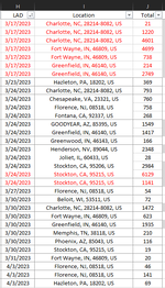
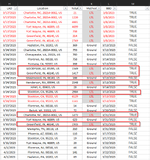
To add reasoning and hopefully clarity to what I'm trying to accomplish; I have a set of Data with Locations and dates and unit totals. (Columns "I", "H", and "J" respectively). In order to know whether to consolidate them, the location must match, the dates must match, and the sum of units from column J must be > 1300. In the attached example, I have already changed font to red to indicate the individual locations would be consolidated as each set of locations has matching dates from column "H") And their total units sum above 1300. Currently I use an if(and(or formula in another column to check if the location and dates match and then I manually sum. So long story short I'm simply trying to combine all into one formula or script.

Example Image: (in this scenario I would need the sum of I2 to I4, the sum of I5 to I6, the sum of I7 to I8).

Any assistance would be greatly appreciated.

 

[awoohaw]

try this:

mr excel questions 13.xlsm
	H	I	J	K
1	LAD	Location
2	2023-03-17	City1	698	TRUE
3	2023-03-17	City1	791	TRUE
4	2023-03-17	City1	646	TRUE
5	2023-03-17	City2	561	TRUE
6	2023-03-17	City2	573	TRUE
7	2023-03-17	City2	770	TRUE
8	2023-03-17	City2	565	TRUE
9	2023-03-24	City3	625	FALSE
10	2023-03-24	City3	638	FALSE
11	2023-03-24	City1	350	FALSE
12	2023-03-24	City1	606	FALSE
13	2023-03-30	City4	643	FALSE
14	2023-03-30	City3	794	TRUE
15	2023-03-30	City3	562	TRUE
Sheet7

Cell Formulas
Range	Formula
K2:K15	K2	=SUMIFS($J$2:$J$15,$H$2:$H$15,H2,$I$2:$I$15,I2)>1300

 

[awoohaw]

Here the formula wrapped in an IF so you can see the sum, i'm showing zero if less than 1300, you can change that to a " " if you want to show blanks:

mr excel questions 13.xlsm
								H	I	J	K	L
1								LAD	Location
2								2023-03-17	City1	698	2135
3								2023-03-17	City1	791	2135
4								2023-03-17	City1	646	2135
5								2023-03-17	City2	561	2469
6								2023-03-17	City2	573	2469
7								2023-03-17	City2	770	2469
8								2023-03-17	City2	565	2469
9								2023-03-24	City3	625	0
10								2023-03-24	City3	638	0
11								2023-03-24	City1	350	0
12								2023-03-24	City1	606	0
13								2023-03-30	City4	643	0
14								2023-03-30	City3	794	1356
15								2023-03-30	City3	562	1356
16
Sheet7

Cell Formulas
Range	Formula
K2:K15	K2	=IF(SUMIFS($J$2:$J$15,$H$2:$H$15,H2,$I$2:$I$15,I2)>1300,SUMIFS($J$2:$J$15,$H$2:$H$15,H2,$I$2:$I$15,I2),0)

 

[lakaihigh]

try this:

mr excel questions 13.xlsm
	H	I	J	K
1	LAD	Location
2	2023-03-17	City1	698	TRUE
3	2023-03-17	City1	791	TRUE
4	2023-03-17	City1	646	TRUE
5	2023-03-17	City2	561	TRUE
6	2023-03-17	City2	573	TRUE
7	2023-03-17	City2	770	TRUE
8	2023-03-17	City2	565	TRUE
9	2023-03-24	City3	625	FALSE
10	2023-03-24	City3	638	FALSE
11	2023-03-24	City1	350	FALSE
12	2023-03-24	City1	606	FALSE
13	2023-03-30	City4	643	FALSE
14	2023-03-30	City3	794	TRUE
15	2023-03-30	City3	562	TRUE
Sheet7

Cell Formulas
Range	Formula
K2:K15	K2	=SUMIFS($J$2:$J$15,$H$2:$H$15,H2,$I$2:$I$15,I2)>1300

This actually works perfectly except for one factor. This will result in "True" even on a single location which requires no consolidation. Example attached.
Is there a way to state that it is false if the location is not a consecutive duplicate? Even if not, this helps tremendously. If I could get it to a point where, it's only showing True on locations that actually contain consecutive duplicates I could simply use conditional formatting to automatically format my data. Currently I'm using a VBA script that I wrote that formats my data (not counting the sum). Then I was manually going back and summing them and removing formatting on ones that shouldn't be formatted. VBA Example for context:

Consolidate()
For Each cell In Sheets(1).Range("I2:I1000" & LastRow)

If (cell.Value = cell.Offset(1, 0).Value Or cell.Value = cell.Offset(-1, 0).Value) And (cell.Offset(, -1).Value = cell.Offset(-1, -1).Value Or cell.Offset(, -1).Value = cell.Offset(1, -1).Value) Then


cell.EntireRow.Interior.Color = 3

End If
Next cell
End Sub

Greatly appreciate the assistance!

 

[awoohaw]

Here you go:

mr excel questions 13.xlsm
								H	I	J	K
1								LAD	Location
2								2023-03-17	City1	698	2135
3								2023-03-17	City1	791	2135
4								2023-03-17	City1	646	2135
5								2023-03-17	City2	561	2469
6								2023-03-17	City2	573	2469
7								2023-03-17	City2	770	2469
8								2023-03-17	City2	565	2469
9								2023-03-24	City3	625	0
10								2023-03-24	City3	638	0
11								2023-03-24	City1	350	0
12								2023-03-24	City1	606	0
13								2023-03-30	City4	1400	0
14								2023-03-30	City3	794	1356
15								2023-03-30	City3	562	1356
Sheet7

Cell Formulas
Range	Formula
K2:K15	K2	=IF(AND(COUNTIFS($H$2:$H$15,H2,$I$2:$I$15,I2)>1, SUMIFS($J$2:$J$15,$H$2:$H$15,H2,$I$2:$I$15,I2)>1300 ),SUMIFS($J$2:$J$15,$H$2:$H$15,H2,$I$2:$I$15,I2),0)

 

[awoohaw]

with counts and true/false:

mr excel questions 13.xlsm
	H	I	J	K	L
1	LAD	Location
2	2023-03-17	City1	698	2135	TRUE
3	2023-03-17	City1	791	2135	TRUE
4	2023-03-17	City1	646	2135	TRUE
5	2023-03-17	City2	561	2469	TRUE
6	2023-03-17	City2	573	2469	TRUE
7	2023-03-17	City2	770	2469	TRUE
8	2023-03-17	City2	565	2469	TRUE
9	2023-03-24	City3	625	0	FALSE
10	2023-03-24	City3	638	0	FALSE
11	2023-03-24	City1	350	0	FALSE
12	2023-03-24	City1	606	0	FALSE
13	2023-03-30	City4	1400	0	FALSE
14	2023-03-30	City3	794	1356	TRUE
15	2023-03-30	City3	562	1356	TRUE
Sheet7

Cell Formulas
Range	Formula
K2:K15	K2	=IF(AND(COUNTIFS($H$2:$H$15,H2,$I$2:$I$15,I2)>1, SUMIFS($J$2:$J$15,$H$2:$H$15,H2,$I$2:$I$15,I2)>1300 ),SUMIFS($J$2:$J$15,$H$2:$H$15,H2,$I$2:$I$15,I2),0)
L2:L15	L2	=AND(COUNTIFS($H$2:$H$15,H2,$I$2:$I$15,I2)>1, SUMIFS($J$2:$J$15,$H$2:$H$15,H2,$I$2:$I$15,I2)>1300 )

 

[lakaihigh]

Here you go:

mr excel questions 13.xlsm
								H	I	J	K
1								LAD	Location
2								2023-03-17	City1	698	2135
3								2023-03-17	City1	791	2135
4								2023-03-17	City1	646	2135
5								2023-03-17	City2	561	2469
6								2023-03-17	City2	573	2469
7								2023-03-17	City2	770	2469
8								2023-03-17	City2	565	2469
9								2023-03-24	City3	625	0
10								2023-03-24	City3	638	0
11								2023-03-24	City1	350	0
12								2023-03-24	City1	606	0
13								2023-03-30	City4	1400	0
14								2023-03-30	City3	794	1356
15								2023-03-30	City3	562	1356
Sheet7

Cell Formulas
Range	Formula
K2:K15	K2	=IF(AND(COUNTIFS($H$2:$H$15,H2,$I$2:$I$15,I2)>1, SUMIFS($J$2:$J$15,$H$2:$H$15,H2,$I$2:$I$15,I2)>1300 ),SUMIFS($J$2:$J$15,$H$2:$H$15,H2,$I$2:$I$15,I2),0)

Absolutely perfect.
Appreciate your time so very much!

 

[awoohaw]

if you have 365 or 2021 version of excel you can even get a filtered output. (You should update your profile to show which version as solutions will vary from version to version of excel).

 

[awoohaw]

happy to help!

 

[lakaihigh]

if you have 365 or 2021 version of excel you can even get a filtered output. (You should update your profile to show which version as solutions will vary from version to version of excel).

Thank you, I will do that. Appreciate your time immensely.