Taking the second derivative of the quadratic fit.

[steve case]

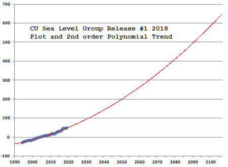
My data looks like this:

1992.960 -31.0
1992.985 -33.1
1993.010 -30.9
1993.039 -33.0
1993.064 -35.8
and so on for 900 lines

Time intervals in column "A" are variable and sometimes missing
and column "B" variables wobble up and down mostly up.

I can easily find acceleration using the slope for the first 450 lines
and the second 450 lines with the formula we all learned in 12th
grade physics (v2-v1)/t=a but it doesn't fly if you let on that that's
what was used to come up with nearly the same answer that taking
the 2nd derivative of the quadratic fit finds. I was never a calculus
student so I need a cook-book answer. I've done an internet search
and a Mr. Excel search and I haven't found anything specific or that
I understand that can be plugged into Excel to find "a" by taking the
2nd derivative of the quadratic.

I'm hoping for X values in column "A" and Y values in Column "B"
with formulas in Columns "C" "D" ... etc. copied on down all the lines
that maybe even give me an answer after the first few rows for a value
of "a" for each row from the beginning (-:

I'm not really asking an Excel question it's more like asking for help
with math. So if that's not what Mr. Excel does, my next step is off to
the the local university and a math tutor. I'm prepared to do that.

 

[Eric W]

What exactly are you trying to do? It appears that you have a set of time/position ordered pairs, and you want to figure out the acceleration from that? And it sounds like you did a quadratic curve fit of the data?

First I'd suggest graphing your points and seeing if it appears to be a continuous function. If not, any value you get out of it will be misleading. Second, try to figure out what type of function might fit best, quadratic, sine, exponential. Keep in mind that the second differential of a quadratic function (the acceleration) is just a constant. If the graph appears to "speed up/slow down", then you'll need a more complex function.

If you can't come up with a suitable function that fits your data reasonably well, you can try "numerical differentiation" (see Wikipedia). Most algorithms that do that require equidistant points, which your data does not have. You'd have to adapt one of the algorithms, or possibly interpolate your data to create the midpoints. And you'd still want some assurance that the underlying function you're trying to map is continuous.

Hope this gives you some ideas.

 

[KRice]

Steve,
I'm curious about the type of data you have. You mentioned taking the slope of the first 450 lines to find acceleration, leading me to believe that you have time/speed ordered pairs, but I'm not sure because you've also mentioned the second derivative (which would imply time/position data). I would caution that finding acceleration from either speed or position data can be, and often is, problematic, especially if beginning with positional data. This is true even for well-behaved systems due to the sensitivity of the derivative to random variations in the measurements (assuming you have experimental data). Evaluating a second derivative only exacerbates this problem, and could yield wildly varying calculated accelerations for what appears to be a well-behaved object under test. For this reason, these type of data are often smoothed, either before differentiation or as part of the differentiation process. I wouldn't necessarily latch onto a quadratic fit, at least not without having a good reason to do so (perhaps a theoretical basis). That would be ideal, because having a functional form generally allows for an analytical expression for the derivative(s). Lacking that, there are many "recipes" for numerical differentiation, but some effort would be needed to assess the variability of the results and determine which approach to take.

 

[steve case]

What exactly are you trying to do? It appears that you have a set of time/position ordered pairs, and you want to figure out the acceleration from that? And it sounds like you did a quadratic curve fit of the data?

First I'd suggest graphing your points and seeing if it appears to be a continuous function. If not, any value you get out of it will be misleading. Second, try to figure out what type of function might fit best, quadratic, sine, exponential. Keep in mind that the second differential of a quadratic function (the acceleration) is just a constant. If the graph appears to "speed up/slow down", then you'll need a more complex function.

If you can't come up with a suitable function that fits your data reasonably well, you can try "numerical differentiation" (see Wikipedia). Most algorithms that do that require equidistant points, which your data does not have. You'd have to adapt one of the algorithms, or possibly interpolate your data to create the midpoints. And you'd still want some assurance that the underlying function you're trying to map is continuous.

Hope this gives you some ideas.

Thanks Eric, I started out thinking this would be simple. Since posting that the
other day, I've done more digging to realize that it apparently isn't simple hence
the silence until your post. I've been engaged in the climate wars for over a
decade and I'm trying to duplicate/figure out how to come up with the same
answer as some of the well recognized academic institutions do. In particular
this one:
Colorado's Sea Level Research Group
Here's their data:
LINK
Here's the link to their paper
LINK
Where they estimate acceleration of sea level rise to be 0.084 ± 0.025 mm/year²
and extrapolate that out to 2100 via the quadratic

Well, it's easy to take the slope of the first and second half of those 894 lines of
data and plug them into the (v2-v1)/t=a formula we all learned in 12th grade
physics and it comes out real close to 0.084 mm/yr² i.e., 0.0846 mm/yr² But when
it was revealed that the 12th grade physics formula was used to verify that, the
comment was:

"Using the (v2-v1)/t=a formula? That’s not how to calculate acceleration.
Take the second derivative of the quadratic fit."

So that's why I wound up here. And it looks like I'm not going get a simple answer and
it's probably unfair of me to press on with it here. After my search these last few days,
I don't hold out much hope for a hired tutor at the local University either. I do have
another source, a close relative that I see once in a while (-:

If I get an Excel answer to all this, I'll post it here.

I'm retired since 2009, but when I was working I built Excel programs full of formulas
and macros for people that did some really neat things. And most of them contained
some VB lines of code supplied by Mr. Excel Dot Com that made the thing work.

​

 

[KRice]

Steve,
Thanks for sharing some details and the links. I had a quick look to try to get you started. I copied the data in your link to columns A and B, inserted a header...and from there the formulas in the example here should allow you to duplicate this trial and investigate some other options. I used the 2nd order fit only because that was the approach taken by the authors. The plot looks very similar to theirs. The quadratic coefficients are reported out by LINEST, and after double differentiation, the acceleration is found to be 0.096 mm/y^2. Some additional work would be needed to investigate confidence intervals and the discrepancy with the authors reported acceleration. I wouldn't necessarily agree that the quadratic fit is appropriate...for example, there may be some cyclical behavior that is obscured by this approach.

MrExcel_problem-solving.xlsx
	A	B	C	D	E	F	G	H	I
1	Time (y)	GMSL (mm)						GMSL = global mean sea level
2	1992.960	-31						Time range of data (y)	25.054
3	1992.985	-33.1
4	1993.010	-30.9						Point estimator with FORECAST
5	1993.039	-33						Time (yyyy.xxx)	2015.355
6	1993.064	-35.8						Est. GMSL (mm)	37.49196
7	1993.096	-36.7
8	1993.119	-34		power of t	2	1	0
9	1993.147	-29.6		GMSL(t)	0.047897	-188.9777	186355.52	quadratic fit of original position/time data
10	1993.175	-28.4				0.095794	-188.9777	1st derivative (speed)
11	1993.202	-28.4					0.095794	2nd derivative (acceleration)
12	1993.229	-29
13	1993.283	-31
14	1993.311	-26.2
15	1993.338	-27.7
16	1993.365	-26.5
17	1993.392	-30.5
18	1993.419	-31
19	1993.446	-28.3
20	1993.474	-25.5
21	1993.501	-25.2
22	1993.528	-25.1
23	1993.582	-30.2
24	1993.610	-29
25	1993.637	-26.2
26	1993.664	-25.2
27	1993.691	-28.1
Sheet18

Cell Formulas
Range	Formula
I2	I2	=MAX(A:A)-MIN(A:A)
I6	I6	=FORECAST(I5,B:B,A:A)
E9:G9	E9	=LINEST(B2:B895,A2:A895^{1,2})
F10:G10	F10	=E8*E9
G11	G11	=F10
Press CTRL+SHIFT+ENTER to enter array formulas surrounded with curly braces.

 

[steve case]

Steve,
Thanks for sharing some details and the links. I had a quick look to try to get you started. I copied the data in your link to columns A and B, inserted a header...and from there the formulas in the example here should allow you to duplicate this trial and investigate some other options. I used the 2nd order fit only because that was the approach taken by the authors. The plot looks very similar to theirs. The quadratic coefficients are reported out by LINEST, and after double differentiation, the acceleration is found to be 0.096 mm/y^2. Some additional work would be needed to investigate confidence intervals and the discrepancy with the authors reported acceleration. I wouldn't necessarily agree that the quadratic fit is appropriate...for example, there may be some cyclical behavior that is obscured by this approach.

MrExcel_problem-solving.xlsx
	A	B	C	D	E	F	G	H	I
1	Time (y)	GMSL (mm)						GMSL = global mean sea level
2	1992.960	-31						Time range of data (y)	25.054
3	1992.985	-33.1
4	1993.010	-30.9						Point estimator with FORECAST
5	1993.039	-33						Time (yyyy.xxx)	2015.355
6	1993.064	-35.8						Est. GMSL (mm)	37.49196
7	1993.096	-36.7
8	1993.119	-34		power of t	2	1	0
9	1993.147	-29.6		GMSL(t)	0.047897	-188.9777	186355.52	quadratic fit of original position/time data
10	1993.175	-28.4				0.095794	-188.9777	1st derivative (speed)
11	1993.202	-28.4					0.095794	2nd derivative (acceleration)
12	1993.229	-29
13	1993.283	-31
14	1993.311	-26.2
15	1993.338	-27.7
16	1993.365	-26.5
17	1993.392	-30.5
18	1993.419	-31
19	1993.446	-28.3
20	1993.474	-25.5
21	1993.501	-25.2
22	1993.528	-25.1
23	1993.582	-30.2
24	1993.610	-29
25	1993.637	-26.2
26	1993.664	-25.2
27	1993.691	-28.1
Sheet18

Cell Formulas
Range	Formula
I2	I2	=MAX(A:A)-MIN(A:A)
I6	I6	=FORECAST(I5,B:B,A:A)
E9:G9	E9	=LINEST(B2:B895,A2:A895^{1,2})
F10:G10	F10	=E8*E9
G11	G11	=F10
Press CTRL+SHIFT+ENTER to enter array formulas surrounded with curly braces.

View attachment 7805

Thanks for all of that. Not to put too fine a point on it, it look like there's a lot of guess work involved.

I am reminded of this quote:

According to physicist Freeman Dyson, the famous mathematician John von Neumann stated: "Give me four adjustable parameters and I can fit an elephant. Give me one more, and I can make his trunk wiggle."

And on that note, thanks for all your effort, but I'm going to call of the hunt for now.

 

[steve case]

One last comment if anyone is interested in this stuff:

From the CU Sea Level Group's 894 lines of data, take the average to come up with 2005.776
Take the difference:
2005.776 minus 1992.96 to come up with t=12.815 and round off to t=12.82
For v1 take the slope A1 to A443 (2005.772) to get 2.8361 and round off to v1=2.84
For v2 take the slope A444 to A894 (2005.772) to get 3.919 and round off to v2=3.92

Plug the values for t, v1, v2 into a=(v2-v10)/t to yield 0.0842 and round off to a=0.084 mm/year²
Which is exactly what CU's Sea Level Group got in their Feb 2018 paper.

The 2nd Order Polynomial plots out to 650 mm ( 65cm ) just like they said.

Here's a quick % Dirty graph of that:

Thank you Eric & KRice for your comments.

 

[Eric W]

That is interesting! However, from a mathematical point of view, extrapolating a curve 5 times further out than your source data is really suspect. There are more variables that we need to consider. In this case, I think it's unlikely that the sea level can continue to rise that much, simply because we'll run out of polar ice to create the water. I'm not a denier, I'm seriously concerned about climate issues, but any flaws in the analysis will be picked apart and the whole argument dismissed. Good luck with your endeavors.

 

[steve case]

That is interesting! However, from a mathematical point of view, extrapolating a curve 5 times further out than your source data is really suspect. There are more variables that we need to consider. In this case, I think it's unlikely that the sea level can continue to rise that much, simply because we'll run out of polar ice to create the water. I'm not a denier, I'm seriously concerned about climate issues, but any flaws in the analysis will be picked apart and the whole argument dismissed. Good luck with your endeavors.

This wonderful forum is not the place to start that discussion. There are plenty of places to critique and discuss such matters.

 

[KRice]

Steve,
Your earlier point about the amount of guesswork is well-taken. This is one reason why the uncertainty analysis presented is so important, but there are still many things in the paper that could and probably should be the subject of further debate.

In the paper, the authors describe their methodology for determining acceleration---a least-squares quadratic fit with points equally weighted (which yielded an acceleration of 0.097 mm/y^2), followed by some "corrections" due to: 1) the Mount Pinatubo eruption in 1991, which is said to have decelerated the GMSL (estimated as -0.02 mm/y^2); and 2) inter-annual variability in terrestrial water storage, mainly driven by El Nino Southern Oscillation (ENSO) effects (estimated as 0.033 mm/y^2). Summing these (0.097 + 0.020 - 0.033) mm/y^2 yields 0.084 mm/y^2, their final reported value. The quick effort in my earlier post used the Excel LINEST formula to perform a 2nd order polynomial regression of the uncorrected GMSL data, which is consistent with the paper's described method. The acceleration obtained, 0.096 mm/y^2, agrees well with the paper's value of 0.097 mm/y^2. But as just mentioned, more information is necessary to arrive at the "corrected" value of 0.084 mm/y^2.

Your most recent post describes how you obtained an acceleration of 0.084 mm/y^2. It appears that that you performed two linear regressions separately on (A1:A443,B1:B443) and (A444:A894,B444:B894) to obtain average velocities for the lower and upper halves of the data set (that's the only way I was able to match the slope values you mentioned). Those two velocities were then used in an equation that essentially yields an average acceleration over the entire curve. It is interesting that this analysis approach results in an acceleration that matches the reported corrected value, but I suspect that it is only coincidental and I don't see anything in the paper to suggest that the authors arrived at their acceleration value this way.

The authors use a "rate of sea-level rise" of 2.9 mm/y, which is considered a point velocity associated with epoch 2005.0. This value was not derived in the paper. So what we can say is that IF a second order equation is a reasonable and valid description of the GMSL over the 25-y period described, and the acceleration is nominally 0.084 mm/y^2 and constant, and the velocity at t=2005.0 was 2.9 mm/y, then we know enough to write some equations. The first coefficient (U4) of the quadratic has a value equal to half of that of the acceleration, and the second coefficient (V4) is determined to satisfy the "known" velocity in 2005. The third coefficient (W4, a constant) sets the initial GMSL "height" at some value...which I arbitrarily set to 0 for t=2005 in the table below. This offers a simple check then on the reported estimated sea-level rise of 654 mm by year 2100.

Reconciliation of effective coefficients for GMSL acceleration & velocity described in Nerem et al. (2018)

MrExcel_problem-solving.xlsx
	U	V	W	X	Y	Z
2	t2	t1	t0
3	2	1	0	<-- exponents year -->	2005	2100
4	0.042	-165.52	163026.6	y, height	0.00	654.55
5		0.084	-165.52	dy/dt, velocity	2.90	10.88
6			0.084	d2y/dt2, acceleration	0.084	0.084
Sheet18

Cell Formulas
Range	Formula
Y4:Z6	Y4	=$U4*Y$3^$U$3+$V4*Y$3^$V$3+$W4*Y$3^$W$3
V5,W5:W6	V5	=U$3*U4

I appreciate having the opportunity to look closer at this complex issue...thanks for sharing, and best of luck with your future work on this.

Kirk