Transferring VBA code to another cell

[Joek88]

Ok, I have wrote a section of code that is fairly long and includes many different cells. My question is this: Can I use the VBA code that I have written and push that code to another cell? I do not just want to simply copy and paste the logic into a cell, but I want the logic to be changed to look a the cells and reformat all the cells to match the new location.

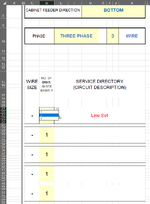
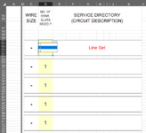
So here is part of my VBA code below. It basically consist of cell D21 with a dropdown selection of 1,2, or 3. It merges and changes cells based on the selection made in the dropdown. However, I want to move the "logic" part of it to D28. Doing this the "old fashion" way, I would have to go through the entire code and change each cell to it's apporiate new location. This is EXTREMELY time consuming and leads to alot of error. There HAS to be an easier way to achieve this. D28 also has the exact dropdown as D21. I want the code to change based on the new location. So this is why a simple copy and paste will not work. Can this be done or am I dreaming? I can provide my entire code if necessary.

Private Sub HandleCase1()

' Merges and unmerges cells based on Case1 being selected

Range("C21:C26").merge
Range("C21").Value = "-"
Range("C21:C26").Borders(xlEdgeBottom).linestyle = xlContinuous
Range("C28:C33").merge
Range("C28").Value = "-"
Range("C28:C33").Borders(xlEdgeTop).linestyle = xlContinuous
Range("C28:C33").Borders(xlEdgeBottom).linestyle = xlContinuous
Range("C35:C40").merge
Range("C35").Value = "-"
Range("C35:C40").Borders(xlEdgeTop).linestyle = xlContinuous
Range("D21:D33").UnMerge
Range("D21:D26").merge
Range("D27").Interior.ColorIndex = xlNone
Range("D21:D26").Borders(xlEdgeBottom).linestyle = xlContinuous
Range("D28:D33").Borders(xlEdgeTop).linestyle = xlContinuous
Range("D28:D33").merge
If Range("D28").Value = "" Then Range("D28").Value = 1
Range("D34").Interior.ColorIndex = xlNone
Range("D35:D40").merge
Range("D28:D33").Borders(xlEdgeBottom).linestyle = xlContinuous
Range("D28:D33").Borders(xlEdgeTop).linestyle = xlContinuous
Range("D35:D40").Borders(xlEdgeTop).linestyle = xlContinuous
If Range("D35").Value = "" Then Range("D35").Value = 1

 

[Joe4]

Please clearly define:
- exactly which cells that you want the code to apply to (list each one)
- explain the logic to be applied, relative to the cell, in plain English

For example, let's say that you wanted to apply this to cells D21, D28, D35, .... D70
And the first part of the logic is to then merge column C of that same row (for whichever of the cells above that is selected) with the next five cells in column C just below it.

If you can plainly specify all those rules, we should be able to come up with code for you.

 

[Joek88]

No problem! I hope I can explain it well enough through pictures and examples to better help you understand what I am trying to achieve. This may be a little lengthy but I'm trusting someone smarter than me can help fix it.

So when I select from D21 dropdown, it shows me 1, 2, or 3. This in turn will basically merge the cells together. See below.

Notice how when I selected a value of 2, it automatically merged the cells together.

And selection 3 merges all three together.

Or if I made a mistake and I want to go back and select 1 when a 3 was already selected. The code will reset it back to the original.

So the VBA code looks at conditions based on the selection of D21 dropdown. The code works flawlessly and exactly how I want it to work. However, I have multiple combinations based on how I select the dropdown. For example, Lets say I have selected a 2 in D21 dropdown. It will merge the cells together down to row 33. Now I want to use this same type of logic and apply it to cell D35. Cell D35 will also have a dropdown that is identical to D21. So if I was to select a value of the following in D35's dropdown it would merge accordingly. Does this make sense? See how there can be multiple scenarios and different combinations based on the dropdown selections.

Essentially I need each cell to act with its own logic like explained above. They go in groups of 7.
For example: D21,D28,D35,D40,....D266

 

[Joe4]

I am still not 100% clear.
(By the way, merged cells in Excel are just about the worst thing out there, and cause all sorts of issues for things like sorting, VBA, etc -- as such, most serious programmers avoid them like the plague!).

Back to your problem, it merges a set number of cells together based on the value selected? Is that correct?
So, it appears that if "1" is selected, it merged 6 rows.
If a "2" is selected, then it merges 13 rows.
And if a "3" is selected, then it merges 20 rows.
Is that all correct?

The "un-doing" is going to be a bit trickier, as I think you may need to know not just what the value was changed to, but what it previously was.
Probably not the way I would try to set this up, but we'll see what we can do with it.

 

[Joek88]

Yes, you are correct! It merges a set number of cells based on the value selected.

This is all correct, yes!
So, it appears that if "1" is selected, it merged 6 rows.
If a "2" is selected, then it merges 13 rows.
And if a "3" is selected, then it merges 20 rows.
Is that all correct?

 

[Joe4]

OK, try this. Right-click on the tab sheet name at the bottom of your sheet, select "View Code", and then place this VBA code in the VB Editor window that pops up (the code NEEDS to be in this location in order to run automatically):

Public prevVal As Variant


Private Sub Worksheet_SelectionChange(ByVal Target As Range)
'   Capture previous values from column D, row multiples of 7 after row

    Dim r As Long

'   See if selected column is column D
    If Target.Column = 4 Then
'       Capture current row
        r = Target.Row
'       See if row is row 21 or below and is a multiple of 7
        If Target.Row >= 21 And (Target.Row Mod 7 = 0) Then
'           Capture current value
            prevVal = Target.Value
        End If
    End If
   
End Sub


Private Sub Worksheet_Change(ByVal Target As Range)
'   Capture previous values from column D, row multiples of 7 after row

    Dim r As Long
    Dim curVal As Long
    Dim prevRng As Range
    Dim curRng As Range

'   See if selected column is column D
    If Target.Column = 4 Then
'       Capture current row and current value
        r = Target.Row
        curVal = Target.Value
'       See if row is row 21 or below and is a multiple of 7
        If (r >= 21) And (r Mod 7 = 0) Then
'           Unmerge column C rows based on previous value
            Set prevRng = Range(Cells(r, "C"), Cells(r + (prevVal * 7) - 2, "C"))
            prevRng.UnMerge
'           Merge colum C rows based on current value
            Set curRng = Range(Cells(r, "C"), Cells(r + (curVal * 7) - 2, "C"))
            curRng.Merge
        End If
    End If
   
End Sub

So, as you update the values in column D in rows 21, 28, 35, 42, 49, etc, it will automatically unmerge/merge the cells in column C.

Note that I just did the merging. But I set range variables named "prevRng" and "curRng" in the code, that you can use to apply other properties to easily.

 

[Joek88]

Hmm, I tried this code and the program is unchanged. Nothing seems to be different in the way it functions. I completely understand the logic of what the code is trying to perform, it's just not performing what the code is asking.

 

[Joe4]

Are you sure that you have placed it in the "Sheet" module of the sheet that it needs to run in?
It absolutely has to be there, and it absolutely needs to be named exactly as shown.
If either of those things are not true, it will not run automatically.

To verify it is firing, add this line just after the title:

Private Sub Worksheet_Change(ByVal Target As Range)
    MsgBox "Code is running..."
    ...

Then, as you update cells, you should see that Message Box pop-up. If you do not, then the code is not being called, which means it is probably in the wrong spot.

If it is running (you get that message), but nothing seems to be happen, then confirm the following:
- what value are you entering?
- what cell are you entering it in?
- are those values text or valid numbers?

 

[Joek88]

Ok I had to rename a sub. I had the ambiguous name error. Once that was changed, the program works.

 

[Joe4]

Ok I had to rename a sub. I had the ambiguous name error. Once that was changed, the program works.

Yes, all event procedures (automated code) have strict naming conventions - there is no flexibility there. They MUST be named a certain way.
And you cannot have two procedures in the same module with the same name.

That fact that you had an "ambiguous name error" tells me that you already had a "Worksheet_Change" event procedure on that sheet. If you renamed the other one, then that one will no longer be automated. You would need to combine both codes into same procedure. You can do that simply by having different code blocks, structured something like this.:

Private Sub Worksheet_Change(ByVal Target As Range)

'***CODE BLOCK 1***
'   Code here

'***CODE BLOCK 2***
'   Code here

End Sub

You just need to be careful if you have any code in your first block that has a line like "Exit Sub", as if it hits that, it would never get to CODE BLOCK2.
You can usually get around that by using IF...THEN blocks for each code block instead.