Hello everyone,
In a sheet named "Anc_Communs", I have three columns: "A", "B" and "C".
1- To begin, we will create a list with unique values from column "A" to column "E". I found a code to do this step, it's working.
2- Next, we will transpose the data from column “B” and column “C” for each cell in column “E”.
Here are the steps to do, for this, I will take an example to better explain to you
We work with the cells of column "E2", we take the value of the first cell of this column: "E2", we find the value of this cell in cells "A2" and "A3", we will therefore transpose the value of cell "B2" into "F2" and the value of "C2" into "G2", then, we transpose the value of cell "B3" into "H2" and the value of "C3" into "I2 "
We then move to the next cell of column "E", this is cell "E3", ", we find the value of this cell in cells "A4" and "A5", we will therefore transpose the value of cell "B4" to "F3" and the value of "C4" to "G3", then we transpose the value of cell "B5" to "H3" and the value of "C5" to "I3" .
Then we continue to do the same thing for all the cells in column “E”.
I started to do this part of code but I'm stuck and I can't move forward, I used tables to make the code faster), I'm putting it at your disposal in the hope that an expert in vba any of you could help me finalize.
Thank you in advance for your contributions.
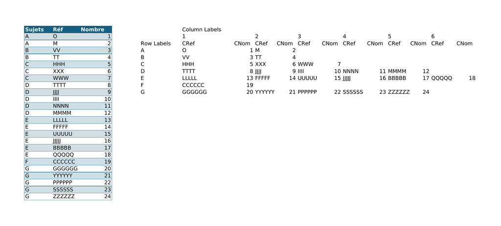
Starting table:
Unless I'm mistaken, here is the final result:
Here is the code I tried to do:
In a sheet named "Anc_Communs", I have three columns: "A", "B" and "C".
1- To begin, we will create a list with unique values from column "A" to column "E". I found a code to do this step, it's working.
2- Next, we will transpose the data from column “B” and column “C” for each cell in column “E”.
Here are the steps to do, for this, I will take an example to better explain to you
We work with the cells of column "E2", we take the value of the first cell of this column: "E2", we find the value of this cell in cells "A2" and "A3", we will therefore transpose the value of cell "B2" into "F2" and the value of "C2" into "G2", then, we transpose the value of cell "B3" into "H2" and the value of "C3" into "I2 "
We then move to the next cell of column "E", this is cell "E3", ", we find the value of this cell in cells "A4" and "A5", we will therefore transpose the value of cell "B4" to "F3" and the value of "C4" to "G3", then we transpose the value of cell "B5" to "H3" and the value of "C5" to "I3" .
Then we continue to do the same thing for all the cells in column “E”.
I started to do this part of code but I'm stuck and I can't move forward, I used tables to make the code faster), I'm putting it at your disposal in the hope that an expert in vba any of you could help me finalize.
Thank you in advance for your contributions.
Starting table:
| compare colonnes.xlsm | |||||
|---|---|---|---|---|---|
| A | B | C | |||
| 1 | Sujets | Réf | Nombre | ||
| 2 | A | O | 1 | ||
| 3 | A | M | 2 | ||
| 4 | B | VV | 3 | ||
| 5 | B | TT | 4 | ||
| 6 | C | HHH | 5 | ||
| 7 | C | XXX | 6 | ||
| 8 | C | WWW | 7 | ||
| 9 | D | TTTT | 8 | ||
| 10 | D | JJJJ | 9 | ||
| 11 | D | IIII | 10 | ||
| 12 | D | NNNN | 11 | ||
| 13 | D | MMMM | 12 | ||
| 14 | E | LLLLL | 13 | ||
| 15 | E | FFFFF | 14 | ||
| 16 | E | UUUUU | 15 | ||
| 17 | E | JJJJJ | 16 | ||
| 18 | E | BBBBB | 17 | ||
| 19 | E | QQQQQ | 18 | ||
| 20 | F | CCCCCC | 19 | ||
| 21 | G | GGGGGG | 20 | ||
| 22 | G | YYYYYY | 21 | ||
| 23 | G | PPPPPP | 22 | ||
| 24 | G | SSSSSS | 23 | ||
| 25 | G | ZZZZZZ | 24 | ||
Anc_Communs | |||||
Unless I'm mistaken, here is the final result:
| Exporter.xlsm | |||||||||||||||||||
|---|---|---|---|---|---|---|---|---|---|---|---|---|---|---|---|---|---|---|---|
| A | B | C | D | E | F | G | H | I | J | K | L | M | N | O | P | Q | |||
| 1 | Sujets | Réf | Nombre | Sujets | |||||||||||||||
| 2 | A | O | 1 | A | O | 1 | M | 2 | |||||||||||
| 3 | A | M | 2 | B | VV | 3 | TT | 4 | |||||||||||
| 4 | B | VV | 3 | C | HHH | 5 | XXX | 6 | WWW | 7 | |||||||||
| 5 | B | TT | 4 | D | TTTT | 8 | JJJJ | 9 | IIII | 10 | NNNN | 11 | MMMM | 12 | |||||
| 6 | C | HHH | 5 | E | LLLLL | 13 | FFFFF | 14 | UUUUU | 15 | JJJJJ | 16 | BBBBB | 17 | QQQQQ | 18 | |||
| 7 | C | XXX | 6 | F | CCCCCC | 19 | |||||||||||||
| 8 | C | WWW | 7 | G | GGGGGG | 20 | YYYYYY | 21 | PPPPPP | 22 | SSSSSS | 23 | ZZZZZZ | 24 | |||||
| 9 | D | TTTT | 8 | ||||||||||||||||
| 10 | D | JJJJ | 9 | ||||||||||||||||
| 11 | D | IIII | 10 | ||||||||||||||||
| 12 | D | NNNN | 11 | ||||||||||||||||
| 13 | D | MMMM | 12 | ||||||||||||||||
| 14 | E | LLLLL | 13 | ||||||||||||||||
| 15 | E | FFFFF | 14 | ||||||||||||||||
| 16 | E | UUUUU | 15 | ||||||||||||||||
| 17 | E | JJJJJ | 16 | ||||||||||||||||
| 18 | E | BBBBB | 17 | ||||||||||||||||
| 19 | E | QQQQQ | 18 | ||||||||||||||||
| 20 | F | CCCCCC | 19 | ||||||||||||||||
| 21 | G | GGGGGG | 20 | ||||||||||||||||
| 22 | G | YYYYYY | 21 | ||||||||||||||||
| 23 | G | PPPPPP | 22 | ||||||||||||||||
| 24 | G | SSSSSS | 23 | ||||||||||||||||
| 25 | G | ZZZZZZ | 24 | ||||||||||||||||
Anc_Communs | |||||||||||||||||||
Here is the code I tried to do:
VBA Code:
Sub Transpose()

'''''############ Create a list without duplicates from column "A" to column "E" ############''''''''

Dim a As Variant, itm As Variant
  Dim d As Object

  Set d = CreateObject("Scripting.Dictionary")
  a = Range("A2", Range("A" & Rows.Count).End(xlUp)).Value
  For Each itm In a
    d(itm) = Empty
  Next itm
  Range("E2").Resize(d.Count).Value = Application.Transpose(d.Keys)

'''''###########################################################################################################''''''''

'''''############ Code to transpose data from column "B" and "C" into rows based on values from column "E" ############''''''''

    Dim Ws As Worksheet
    Dim rng_E As Range, rng_A As Range
    Dim LRow_E As Long, LRow_A As Long
    Dim i As Long, j As Long, n As Long
    Dim Array_E, Array_A, TempAr() As String
    Dim boolFound As Boolean

    Set Ws = ThisWorkbook.Sheets("Anc_Communs")

    LRow_E = Ws.Cells(Rows.Count, "E").End(xlUp).Row
    LRow_A = Ws.Cells(Rows.Count, "A").End(xlUp).Row

    Set rng_E = Ws.Range("E2:E" & LRow_E)
    Set rng_A = Ws.Range("A2:A" & LRow_A)

    Array_E = rng_E.Value
    Array_A = rng_A.Value

    For i = LBound(Array_E) To UBound(Array_E)
        For j = LBound(Array_A) To UBound(Array_A)
            If Array_E(i, 1) = Array_A(j, 1) Then
                boolFound = False
                Exit For
            End If
        Next j

        If boolFound = True Then
            ReDim Preserve TempAr(n)
            TempAr(n) = Array_A(i, 1)
            n = n + 1
        Else
            boolFound = False
        End If
    Next i

    m = 2
      Ws.Cells(m + 1, 6).Resize(UBound(TempAr) + 1, 6).Value = Application.Transpose(TempAr)
'    Ws.Cells(LRow_E + 1, 1).Resize(UBound(TempAr) + 1, 1).Value = Application.Transpose(TempAr)

'''''###########################################################################################################''''''''

End Sub