Unpivot Pairs of Data, however one column per pair is not a value but a text entry

[Yolandi Drossopoulos]

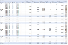
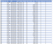
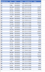
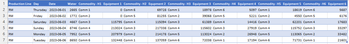
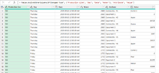
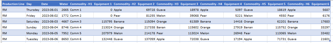
Column 1 - 4 is relevant to all potential data rows. Column 5 - 16 is made up of pairs of data where the first column of the pair is text and the second column for the pair is a value. Very compounded data. See Screen Shots for Possible Data Set. Neither Unpivot and Group By works in this instance, since the pairs are not all values. I will change the data in Excel to try and demonstrate the expected end result, I need assistance to do this in Power Query. There are 4 images. Example of possible original data "Original Data Set", Reworked Dataset (here I did a considerable amount of time to get it into this format, This is what I in essence want to do in Power Query. Tab 3 - PQ Data Table (after some work done in Power Query. Tab 4 - Pivot. In the end I must be able to slice and dice as I need to. Please Help with a possible solution. Please ask any questions if this is not clear. Screen Shot 1 - Possible Original Data Set, Screen Shot 2 End Result Pivot with expectation. Screen Shot 3 - Power Query Transformed Data Set. Screen Shot 4 - Manually changed data set to be able to do expected Pivot Table - Kind Regards. Yolandi Drossopoulos

 

[Yolandi Drossopoulos]

I would be more that willing to provide further information if someone can help me with this problem. I have managed to do this in a way, but am sure there is a better way of doing this. In short what I have done to resolve this at the moment is: I duplicated the Table, Then I kept the initial 1 - 4 columns and deleted columns that starts with commodity and kept just the ones starting with Equipment, I then unpivoted these columns for Equipment. Next I went to the duplicated table and there I kept the columns that starts with Commodity and unpivoted these columns. I then had to do some work to create a lookup key (primary key) to allow me to merge the two tables and bring in some of the required data. Please let me know if there is an easier way to accomplish this. Your input or responses are appreciated. Kind Regards - Yolandi

 

[RoryA]

Unpivot all the column pairs. Parse the Attribute column created so that you have a type (Commodity/Equipment) and the number off the end, then repivot on the Type column.

 

[Yolandi Drossopoulos]

Hi Rory, Thank you for responding. I am not very familiar with the parse function in Power Query. However, I gave what I understood by you solution a go. I just need to understand something in order to explain myself. I brought the original data set into Power Query, herewith a snapshot of original data (Just change some of the naming conventions to fruits in the Commodity Columns to be able to differentiate a bit easier

I then Unpivoted Columns E - P. This is the result

I tried to use the Parse function in Power Query, it gives me two options XML or Jason and on both I got errors returned in the added column. What I need is for the attribute column to have for each line where there is a value the combination of the two lines in attribute as well as the text string in the value column. Just a bit more context : line one and two should be 1 line with a combination of "Commodity - H1, Guava, Equipment 1 (in the Attribute Column) and in this Case the Value Column should have value 0. From here I would then be able to split out the values that I need to group by.
I hope this clarifies my problem a bit better. Your assistance is appreciated. Kind Regards - Yolandi

 

[RoryA]

Sorry, I didn’t actually mean the Parse function in PQ, I meant it in the more traditional sense. You need to extract the text before the first space into one column and the text after it into another, then replace “- H” in the second column with nothing so you just have numbers left. Then pivot the first column, and choose not to aggregate values.

 

[Yolandi Drossopoulos]

Apologies for my late response. Sorry I am a bit stupid with my understanding. Can I just try and confirm in steps what I need to do.

Step 1

Bring the Original Source Data into Power Query

Then I take column E - P and Unpivot (See below is the results after unpivoting column E - P

From here I do not understand your suggestion as to how to get row three and four to become one row with the text circled in red into one column and the associated value in another. If I can get a way to get the text in the circles into one column, I can extract the values that I want to use. In the end I need to have one line with the text as circle in red and the associated value in a next column for the same line. I hope this clarifies my problem

 

[RoryA]

Select the Attribute column, then on the Home tab choose Split column, then By delimiter:

Then in the dialog that appears, choose Space as the delimiter and split at the left-most occurrence:

which will make this:

Select the Attribute.2 column and select the Replace Values button on the Home tab. Enter a dash followed by a space then H and leave the replacement box blank:

Which will leave the Attribute.2 column with just numbers in it:

Select the Attribute.1 column and choose Pivot column on the Transform tab. In the dialog specify Value as the Value field, click the Advanced options dropdown and specify Don't aggregate:

That produces this:

 

[Yolandi Drossopoulos]

Hi Rory, than you for your response and the effort that you took to try and assist. This does not help me in the end, purely because I still need the references to Attribute 1 created in your first step. In short what I did in the end to resolve this is I duplicated the Table.
Then I reordered the columns to have all columns for commodity and sitting next to each other and deleted the Equipment columns in the one table and in the next table I reordered to have all Equipment in the other table. I added an index Column on the two tables as well. Then I unpivoted the data on both the tables and created a Lookup Key using the Index Number and another reference field that I extracted to allow me to then Merge the two tables bringing in all the necessary fields. Doing this then expanded my dataset to have all the necessary values per line. My apologies if I did not explain my problem correctly. Here is a snapshot with what I ended up per value line item.

The data above is with other naming conventions as per my requirements.

Let me know if you know of an easier way to do this. Else, I will close this request.

Again, thank you very much for your response. Have a nice day.

Kind Regards


Yolandi Drossopoulos

 

[RoryA]

I guess I don't understand what you want then, I'm afraid. It would be much easier in future if you could post usable samples (e.g. using XL2BB, or a link to a file somewhere) of the actual data instead of pictures of parts of it.

 

[Yolandi Drossopoulos]

I guess I don't understand what you want then, I'm afraid. It would be much easier in future if you could post usable samples (e.g. using XL2BB, or a link to a file somewhere) of the actual data instead of pictures of parts of it.

Thank you for your time, it is just that sometimes the data is sensitive. I replicated it with example data i.e the fruits.