Using PROCH and PROCV at the same time to find value

[Auctor Somnium]

So I have two spreadsheets:

MAIN:

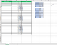
PRODUCTION:

A bit of my situation:
This spreadsheets are examples in the actual one I can't change their structure so a solution has to be through a formula.

I have to do a two condition search, the problem is one is using PROCH and the other is using PROCV (At least this are the only methods I know on how to do this other than PROCX, that I think won't be useful in this situation).


Issue:
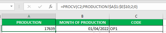
I need the production value to appear in column A of the "MAIN" sheet

The first condition is the month of production, I need to search the "PRODUCTION" sheet and come back with a value according to the month
The second condition is the code, I need to search it there as well and come back with a value according to it

The problem is I have to search an specific column or an specific line index and those are dependant in eachother

In this PROCV for example the PROCH would be the one that would actually define which column it's searching the value in, instead of it searching in this example column 2.The problem is that, doing that doesn't work since the PROCH would also have a line index which would have to be defined by the PROCV it's defining.

Is there any way to do this even with a different formula or manner? Or maybe even with this same formulas but in a way I don't know about

Sorry if it's slightly confusing I can try explaining it better if necessary

 

[Leo Skywalker]

Hi there,

I guess you're using the portuguese version of Excel.


Please, try this formula, in A2:

=ÍNDICE(PRODUCTION!$B$2:$E$10;CORRESP(MAIN!C2;PRODUCTION!$A$2:$A$10;0);CORRESP(MAIN!B2;PRODUCTION!$B$1:$E$1;0))

Which I expect to bethe correct translation of the formula:

=INDEX(PRODUCTION!$B$2:$E$10;MATCH(MAIN!C2;PRODUCTION!$A$2:$A$10;0);MATCH(MAIN!B2;PRODUCTION!$B$1:$E$1;0))

 

[Auctor Somnium]

Hi there,

I guess you're using the portuguese version of Excel.


Please, try this formula, in A2:

=ÍNDICE(PRODUCTION!$B$2:$E$10;CORRESP(MAIN!C2;PRODUCTION!$A$2:$A$10;0);CORRESP(MAIN!B2;PRODUCTION!$B$1:$E$1;0))

Which I expect to bethe correct translation of the formula:

=INDEX(PRODUCTION!$B$2:$E$10;MATCH(MAIN!C2;PRODUCTION!$A$2:$A$10;0);MATCH(MAIN!B2;PRODUCTION!$B$1:$E$1;0))

Thank you it's exactly what I needed

 

[Leo Skywalker]

You're welcome!, Glad that I could help.