Using SUMIFS but have ranges dynamic and extend based on cell row I specify

[hassan023]

Hello all,
I'm hoping I could get help with a specific formula.
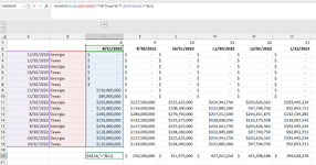
I have a simple SUMIFS formula. I have the SUMIFS formula in the screenshot below.

Column A _criteria 1 : its dates and row 2 is the date requirement (less than)
Column B_criteria 2: text containing *Texas*
and the sum range moves as I copy the formula

The problem is, my model has circular references and I need to change the formula to dynamic range.

Example:
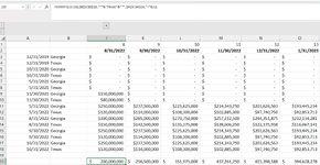
The screen shot is only a few rows but it goes to around 150 rows.
Instead of selecting A3:A150 , B3:150 , J3:J150
I need something that will do A3: but the end range will be based on the current sum range date

so for column J , date is August , given that my criteria is "<" 8/31/2022 , I need the range to from A3:A12 and B3:B12 and J3:J12
Then for column K it will be A3:A12 and B3:B12 and K3:K12

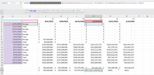
Selecting the whole range gives me a circular reference because I have other tabs linked.

Is there a way to tell it how many rows to go down for the range?
I thought of using Match to get the row number but it still need to select the whole range in MATCH but I think it won't give a circular reference because the SUMIFS range will end up being limited to specific row
I just did not know how to combine A3: with match to get to A12 end rage and so on.

I was thanking maybe , offset counta or match would work?

 

[hassan023]

I was able to come up with a formula but it works only if the date in ROW 2 is available in column A
I need it to sum everything before that date.
Example Column M has date 11/30/2022 , it should sum values up to row 18 with criteria TEXAS

Here is the formula

=SUMIFS(M$3:OFFSET(M$2,MATCH(M$2,$A$3:$A$18,0),),$B$3:OFFSET($B$2,MATCH(M$2,$A$3:$A$18,0),),"*"&"Texas"&"*",$A$3:OFFSET($A$2,MATCH(M$2,$A$3:$A$18,0),),"<"&M$2)

		8​	9​	10​	11​	12​	13​
		8/31/2022​	9/30/2022​	10/31/2022​	11/30/2022​	12/31/2022​	1/31/2023​
12/31/2019​	Georgia	$ -	$ -	$ -	$ -	$ -	$ -
12/31/2019​	Texas	$ -	$ -	$ -	$ -	$ -	$ -
10/31/2020​	Georgia	$ -	$ -	$ -	$ -	$ -	$ -
10/31/2020​	Texas	$ -	$ -	$ -	$ -	$ -	$ -
5/31/2021​	Georgia	$ -	$ -	$ -	$ -	$ -	$ -
5/31/2021​	Texas	$ -	$ -	$ -	$ -	$ -	$ -
11/30/2021​	Georgia	$ 150,000,000	$ -	$ -	$ -	$ -	$ -
11/30/2021​	Texas	$ 80,000,000	$ -	$ -	$ -	$ -	$ -
5/31/2022​	Georgia	$250,000,000​	$237,500,000​	$225,625,000​	$214,343,750​	$203,626,563​	$193,445,234​
5/31/2022​	Texas	$120,000,000​	$114,000,000​	$108,300,000​	$102,885,000​	$97,740,750​	$92,853,713​
8/31/2022​	Georgia	$300,000,000​	$285,000,000​	$270,750,000​	$257,212,500​	$244,351,875​	$232,134,281​
8/31/2022​	Texas	$150,000,000​	$142,500,000​	$135,375,000​	$128,606,250​	$122,175,938​	$116,067,141​
9/30/2022​	Georgia	$250,000,000​	$237,500,000​	$225,625,000​	$214,343,750​	$203,626,563​	$193,445,234​
9/30/2022​	Texas	$120,000,000​	$114,000,000​	$108,300,000​	$102,885,000​	$97,740,750​	$92,853,713​
10/31/2022​	Georgia	$250,000,000​	$237,500,000​	$225,625,000​	$214,343,750​	$203,626,563​	$193,445,234​
10/31/2022​	Texas	$120,000,000​	$114,000,000​	$108,300,000​	$102,885,000​	$97,740,750​	$92,853,713​
		$ 200,000,000	$ 256,500,000	$ 351,975,000	$ 437,261,250	$ 415,398,188	$ 394,628,278
		$ 200,000,000	$ 256,500,000	$ 351,975,000	#N/A​	#N/A​	#N/A​

 

[hassan023]

wow that was an easy I guess I did not need to post this here , I was able to figure it out myself haha

using 1 instead of 0 as match type fixes it

=SUMIFS(M$3:OFFSET(M$2,MATCH(M$2,$A$3:$A$18,1),),$B$3:OFFSET($B$2,MATCH(M$2,$A$3:$A$18,1),),"*"&"Texas"&"*",$A$3:OFFSET($A$2,MATCH(M$2,$A$3:$A$18,1),),"<"&M$2)

Please disregard this thread all. No help needed anymore.