#VALUE using SUMPRODUCT or FILTER

[WSBirch]

Good morning,
I can't for the life of me find what the issue is here and get rid of the #VALUE error.

I'm using this SUMPRODUCT fuction:

=SUMPRODUCT(('Feb 23'!C4:C100=TODAY())*('Feb 23'!D3:AE3="1ST LEAD")*'Feb 23'!D4:AE100)

and I've even tried using this using the filter function:

=SUM(FILTER(FILTER('Feb 23'!D4:AE100,'Feb 23'!C3:AE3=TODAY(),0),'Feb 23'!C4:C100="1ST LEAD",0))

, but in either case, they both return #VALUE.

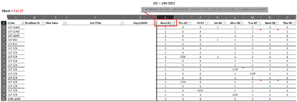
This is in use for an attendance sheet, where if one is present they are marked with a 1. I'm trying to sum those 1's based on today's date on a sheet based on the current month. I intend to eventually adjust the formula to replace the sheet reference with an INDIRECT function to reference any new month sheet we add.

In any case, there's a column of data that marks what Shift & Position is being accounted for per person [C4:C100] (ie. there's 3x 1ST LEAD positions, all are present). There's a row of data that's simply every date of the month excluding Sundays and holidays - it's an array function that displays this [D4:AH4], being:

{=(WORKDAY.INTL(G1-1,SEQUENCE(1,(VLOOKUP(G1,Codes!D:E,2,FALSE))),11,Holidays!A2:A100))}

There is, however, one issue with this array where it's been extended from H3 all the way out to AH3 so that it could capture every day of the month on months with 31 days and any that have less - but in any months where there's less than 31 days the values return #N/A - which I can't seem to remove probably unless I knew a formula to use that wasn't an array here.

None of the data in Column C is formatted a "Text". It's all formatted "General". The data in row 3 are all formatted as a "Custom Date", except for the last few dates where it returns #N/A due to the array formula, but the SUMPRODUCT or FILTER functions I'm trying to use aren't referencing those columns (AF, AG, AH), so I assume it shouldn't matter?

 

[RoryA]

Is there anything in D4:AE100 that is not a number?

 

[WSBirch]

Is there anything in D4:AE100 that is not a number?

There are. There's a number of blank cells throughout the whole range, as not all folks have a "position ID" and cells in the columns for the dates will be left blank for those not in attendance or utilize other codes than numbers like "COS", "COP", "PTO", etc. D4:G100 alone is only text, formatted as "General", or Hire Dates formatted as "Dates".

 

[RoryA]

You can't multiply by text, hence the error. Try something like:

=SUMPRODUCT(('Feb 23'!C4:C100=TODAY())*('Feb 23'!D3:AE3="1ST LEAD")*(IFERROR('Feb 23'!D4:AE100+0,0)))

 

[Fluff]

Judging by the image I think that the Op has the sumproduct ranges the wrong way round.
It looks as though "1ST LEAD" should be col C & row 3 should be Today()

 

[WSBirch]

You can't multiply by text, hence the error. Try something like:

=SUMPRODUCT(('Feb 23'!C4:C100=TODAY())*('Feb 23'!D3:AE3="1ST LEAD")*(IFERROR('Feb 23'!D4:AE100+0,0)))

Interesting, that does remove the issue with #VALUE, but it's not returning the correct value. I just results in "0", where I should be seeing a "3" (since there's 3x 1ST LEADS in attendance today).
But... I wouldn't worry about that.... Fluff here answered my stupid question....

Judging by the image I think that the Op has the sumproduct ranges the wrong way round.
It looks as though "1ST LEAD" should be col C & row 3 should be Today()

Wow... I mean, biggest facepalm... yeah, that fixed it here. Actually both responses fixed it. I needed that IFERROR bit + also swap the terms in the formula... thank you. I feel super dumb!