Value within percentage range

JS050

New Member
Joined
Feb 1, 2023
Messages
7
Office Version
  1. 365
Platform
  1. MacOS
Hi all,

I have been reading a lot of great answers on this forum already, but I can't seem to find the answer to the problem I am facing now.

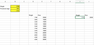
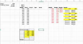
In B2 I have the weight of wood in KG, for example. In B3 &B4 I have the range for which I would like the range to be (+10% & -10%). In D8:D17 is the range of wood in KG with the corresponding prices in E8:E17.

1. How do I get all the values within the + 10% & -10% in the cell I7 and below? Within the range of of D8:D17 there are some the same as the searching value and some are not the same. I have used =(INDEX($D$7:$D$17;MATCH($B$2;$D$7:$D$17;0);(ABS($B$2-$D$7:$D$17)<=ABS($B$2*$B$3))-(ABS($B$2-$D$7:$D$17)<=ABS($B$2*$B$4)))) and it only gives me 3700 as a returning value. Can somebody explain why?
2. How to I get the corresponding prices that go along with the wood in KG in J7 and down?

Thank you very much and much appreciated!
 

Attachments

  • Schermafbeelding 2023-02-01 om 20.44.39.png
    Schermafbeelding 2023-02-01 om 20.44.39.png
    95.5 KB · Views: 9

Excel Facts

Last used cell?
Press Ctrl+End to move to what Excel thinks is the last used cell.
Like this??
Book1
ABCDEFGHI
1
2Weight3700
3Procentual range90%
4110%
5WeightPrice
637002000WeightPrice
73000150037002000
83240150037002000
93240160034501900
103240180037002000
113700200040002500
1234501900
1337002000
1440002500
1543001900
1642002500
Sheet2
Cell Formulas
RangeFormula
H7:I11H7=FILTER(D6:E16,(D6:D16>=B2-(B2*0.1))*(D6:D16<=(B2*1.1)),"Out of Rnge")
Dynamic array formulas.
 
Upvote 0
Like this??
Book1
ABCDEFGHI
1
2Weight3700
3Procentual range90%
4110%
5WeightPrice
637002000WeightPrice
73000150037002000
83240150037002000
93240160034501900
103240180037002000
113700200040002500
1234501900
1337002000
1440002500
1543001900
1642002500
Sheet2
Cell Formulas
RangeFormula
H7:I11H7=FILTER(D6:E16,(D6:D16>=B2-(B2*0.1))*(D6:D16<=(B2*1.1)),"Out of Rnge")
Dynamic array formulas.
Hi AhoyNC,

Thanks a lot for the great suggestion. Unfortunately, at work, we do not have the =filter function... Think we do not have the right Excel for that

Is there any other option you can think of?

In the meantime I have come up with the following: I have used =IF(AND($D$6:$D$16>=$B$2*$B$3;$D$6:$D$16<=$B$2*$B$4);$D$6:$D$16) in cells M6:M15 to only give the values within the 0,975 en 102,5 range. In cells N6:N15 the price is given accordingly with =IF.ERROR(VERT.ZOEKEN(M6;$D$6:$E$16;2;0);"ONWAAR"). (Onwaar = False)

But now I would like to have a summary of all the values, so not the false-values in D20: F27 like in the picture below. I have manually added the values, but what formula would accomplish this? I have tried to download the XL2BB, but unfortunately I can't get that to work..

Thanks again!
 

Attachments

  • Schermafbeelding 2023-02-05 om 13.28.29.png
    Schermafbeelding 2023-02-05 om 13.28.29.png
    249.3 KB · Views: 9
Upvote 0
Does this help. Should work with Excel 2010 and up.
Just drag formula down the row.
Book1
ABCDEFGHI
1
2Weight3700
3Procentual range90%
4110%
5WeightPriceWeightPrice
63700200037002000
73000150037002000
83240150034501900
93240160037002000
103240180040002500
1137002000
1234501900 
1337002000 
1440002500
15 43001900
16 42002500
Sheet1
Cell Formulas
RangeFormula
H6:I10H6=IFERROR(INDEX($D$6:$E$16,AGGREGATE(15,6,(ROW($D$6:$D$16)-ROW($D$6)+1)/(($D$6:$D$16>=$B$2*$B$3)*($D$6:$D$16<=$B$2*$B$4)),ROWS($K$7:K7)),0),"")
H12:H13H12=IFERROR(INDEX($D$6:$E$16,AGGREGATE(15,6,(ROW($D$6:$D$16)-ROW($D$6)+1)/(($D$6:$D$16>=$B$2*$B$3)*($D$6:$D$16<=$B$2*$B$4)),ROWS($K$7:K12)),0),"")
B15:B16B15=IF(AND(D15>$F$1,D15<=$G$1),"T","")
Dynamic array formulas.
 
Upvote 0
Just use the formula in cell H6 above. It picked up some formulas I was just testing with in H12 and B15, that I didn't delete.
 
Upvote 0
Just use the formula in cell H6 above. It picked up some formulas I was just testing with in H12 and B15, that I didn't delete.
Thank you very much for your swift reply!! Where is this part of the formula for : ,ROWS($K$7:K7)),0),"")?
 
Upvote 0
Still don't know where this: ,ROWS($K$7:K7)),0),"") is for but the formula works!!! Thank you so much for your help!
 
Upvote 0
The ROWS($K$7:K7) is just a counter for the SMALL function. It doesn't really mater, but I meant for it to start in cell H6. I was working on different formulas and some got copied over into what I sent to you.

So, ROWS($H$6:H6) will give 1 in the first cell and then 2 in the next cell down. This just tells the SMALL function to pick the 1,2,3 etc. values that match.
The 0 in ROWS($K$7:K7)),0) tells the INDEX to look at all values in the column.
The "" is for the IFERROR function to return a blank cell if there is an error. As you keep dragging the formula down, once it runs out of values to return you would get a #NUM error.

Here is a cleaner copy.
Book1
ABCDEFGHI
1
2Weight3700
3Procentual range90%
4110%
5WeightPriceWeightPrice
63700200037002000
73000150037002000
83240150034501900
93240160037002000
103240180040002500
1137002000
1234501900
1337002000
1440002500
1543001900
1642002500
Sheet1
Cell Formulas
RangeFormula
H6:I10H6=IFERROR(INDEX($D$6:$E$16,AGGREGATE(15,6,(ROW($D$6:$D$16)-ROW($D$6)+1)/(($D$6:$D$16>=$B$2*$B$3)*($D$6:$D$16<=$B$2*$B$4)),ROWS($H$6:H6)),0),"")
Dynamic array formulas.
 
Upvote 0
Solution

Forum statistics

Threads
1,215,043
Messages
6,122,816
Members
449,095
Latest member
m_smith_solihull

We've detected that you are using an adblocker.

We have a great community of people providing Excel help here, but the hosting costs are enormous. You can help keep this site running by allowing ads on MrExcel.com.
Allow Ads at MrExcel

Which adblocker are you using?

Disable AdBlock

Follow these easy steps to disable AdBlock

1)Click on the icon in the browser’s toolbar.
2)Click on the icon in the browser’s toolbar.
2)Click on the "Pause on this site" option.
Go back

Disable AdBlock Plus

Follow these easy steps to disable AdBlock Plus

1)Click on the icon in the browser’s toolbar.
2)Click on the toggle to disable it for "mrexcel.com".
Go back

Disable uBlock Origin

Follow these easy steps to disable uBlock Origin

1)Click on the icon in the browser’s toolbar.
2)Click on the "Power" button.
3)Click on the "Refresh" button.
Go back

Disable uBlock

Follow these easy steps to disable uBlock

1)Click on the icon in the browser’s toolbar.
2)Click on the "Power" button.
3)Click on the "Refresh" button.
Go back
Back
Top