Pinaceous
Well-known Member
- Joined
- Jun 11, 2014
- Messages
- 1,113
- Office Version
- 365
- Platform
- Windows
Good Day All,
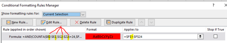
I'm trying to work on a code, where if a row has data in Columns B:E & G, and any information contained from that rows Column H:Z that when Column F is blank under these conditions that its interior cell color will turn red.
Likewise, if under this conditions Column F is not blank, the code will do nothing.
Please note, that this proposed criterion ignores Column A's information.
Can someone help me sort out a VBA for this?
Thank you in advance!
Respectfully,
pinaceous