VBA code to multiply many rows with some conditions

[tennis07]

Hello guys,
please could anyone help me to get the result below:

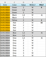
For each day I have 3 columns: color, value and result.
I need to multiply each row of the column value if the date is the same, the color is the same and the result is W.
Eg. For the first 3 rows I have the same date (01/01/2024), the same color (Green) and all the rows = W. So I multiply 2 * 1,5 * 2 and show the result on the first line of this block (Column MULT), which is 6.
If for example I had the first 3 rows with at least one result = L, then, the first line of this block (Column MULT) would be -1. Then I need to do it for all the rows that I have data on my sheet.
I believe the image helps to understand better what I want to explain.

Thanks a lot guys!
Hope someone could help me.

 

[MountainFog]

Just to clarify, If there ever is a L on that day for that color, the result is always -1?

 

[MountainFog]

I wouldn't use VBA. Assuming the data is in A:E, then the following should work. Note you will have to change the ranges to select all your data.

=LET(a,FILTER($C$2:$D$21,($A$2:$A$21=$A2)*($B$2:$B$21=$B2)),b,IF(a="L",1,a),IF(OR($A2<>$A1,$B1<>$B2),IF(SUM(CHOOSECOLS(b,2))>0,-1,PRODUCT(b,1)),""))

 

[tennis07]

Just to clarify, If there ever is a L on that day for that color, the result is always -1?

exactly mate!

 

[tennis07]

View attachment 109593

I wouldn't use VBA. Assuming the data is in A:E, then the following should work. Note you will have to change the ranges to select all your data.

=LET(a,FILTER($C$2:$D$21,($A$2:$A$21=$A2)*($B$2:$B$21=$B2)),b,IF(a="L",1,a),IF(OR($A2<>$A1,$B1<>$B2),IF(SUM(CHOOSECOLS(b,2))>0,-1,PRODUCT(b,1)),""))

Trying to understand the formula you used, its kind of impossible to me.
Thanks a lot.

 

[MountainFog]

Formula only runs when the date changes or color changes from the previous row, otherwise blank.
Takes range C2:D21 and filters it to just that date and color
Changes any L's to 1 to create a condition that if L exists in the second column of the filtered range, equates to -1
Otherwise, multiplies the first column values of filtered range together.

 

[DanteAmor]

Another option with a formula for versions prior to 365. (I recommend you update your Account details to know what Excel version you are using)

varios 06abr2024.xlsm
	A	B	C	D	E	F
1		Date	Color	Value	Result	Mult
2		01-ene	Green	2	W	6
3		01-ene	Green	1.5	W
4		01-ene	Green	2	W
5		01-ene	Black	1.5	W	-1
6		01-ene	Black	2	L
7		01-ene	Yellow	2	W	2
8		01-ene	Red	2	W	16
9		01-ene	Red	2	W
10		01-ene	Red	2	W
11		01-ene	Red	2	W
12		02-ene	Blue	1.5	W	-1
13		02-ene	Blue	1.5	L
14		02-ene	Grey	1.5	W	-1
15		02-ene	Grey	2	W
16		02-ene	Grey	2	W
17		02-ene	Grey	2	W
18		02-ene	Grey	3	W
19		02-ene	Grey	3	L
20		02-ene	Grey	3	W
21		02-ene	Grey	3	W
Hoja2

Cell Formulas
Range	Formula
F2:F21	F2	=IF(COUNTIFS($B$2:B2,B2,$C$2:C2,C2)=1,IF(COUNTIFS(B:B,B2,C:C,C2,E:E,"L"),-1,PRODUCT(D2:INDEX($D$2:$D$21,LOOKUP(2,1/(($B$2:$B$21=B2)*($C$2:$C$21=C2)),ROW($D$2:$D$21))-2+1))),"")

With vba:

Sub MultiplyRows()
  Dim lr As Long
  lr = Range("E" & Rows.Count).End(3).Row
  With Range("F2:F" & lr)
    .Formula = _
        "=IF(COUNTIFS($B$2:B2,B2,$C$2:C2,C2)=1,IF(COUNTIFS(B:B,B2,C:C,C2,E:E,""L""),-1," & _
        "PRODUCT(D2:INDEX($D$2:$D$" & lr & ",LOOKUP(2,1/(($B$2:$B$" & lr & "=B2)*($C$2:$C$" & lr & "=C2)),ROW($D$2:$D$" & lr & "))-2+1))),"""")"
    .Value = .Value
  End With
End Sub

Regards
Dante Amor