VBA & Conditional Formatting

[th259]

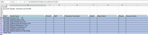
I have a table that was pasted values from a pivot table. The first and second column (Fund and Vendor Name columns) have subtotals. I have the following code to highlight any subtotal rows for column A, but how do I do it for column B?

Dim myRange As Range
    Set myRange = ThisWorkbook.Worksheets("Summary").Range("A6:J" & Range("J" & Rows.Count).End(xlUp).Row)
    With myRange.Borders
    .LineStyle = xlContinuous
    .ColorIndex = 0
    .TintAndShade = 0
    .Weight = xlThin
    End With
    With myRange
        .FormatConditions.Delete
        .FormatConditions.Add Type:=xlExpression, Formula1:="=AND(NOT(ISBLANK($A6)),ISBLANK($E6))"
           .FormatConditions(.FormatConditions.Count).Interior.Color = 15189684
        End With
    myRange.Select
    Selection.AutoFilter
    ActiveSheet.myRange.AutoFilter Field:=2, Criteria1:=RGB(180, 198, 231), Operator:=xlFilterCellColor
End Sub

I had tried the code below and it didn't work.

With myRange
        .FormatConditions.Delete
        .FormatConditions.Add Type:=xlExpression, Formula1:="=SEARCH (" * Total * ", $B6)"
           .FormatConditions(.FormatConditions.Count).Interior.Color = 11854022
        End With

Also, how do I filter the Fund column (column A) to only show the rows with the specific blue fill color and delete the word Total from only those filtered rows then add a vlookup formula in column B only for those filtered rows.

 

[th259]

With myRange
   .FormatConditions.Add Type:=xlExpression, Formula1:="=SEARCH (" * Total * ", $B6)"
   .FormatConditions(.FormatConditions.Count).Interior.Color = 11854022
End With

Why does the code above not work?

 

[th259]

Dim myRange As Range
    Set myRange = ThisWorkbook.Worksheets("Summary").Range("A6:J" & Range("J" & Rows.Count).End(xlUp).Row)
    With myRange.Borders
    .LineStyle = xlContinuous
    .ColorIndex = 0
    .TintAndShade = 0
    .Weight = xlThin
    End With
    With myRange
        .FormatConditions.Delete
        .FormatConditions.Add Type:=xlExpression, Formula1:="=AND(NOT(ISBLANK($A6)),ISBLANK($E6))"
        .FormatConditions(1).Interior.Color = 15189684
        .FormatConditions.Add Type:=xlExpression, Formula1:="=SEARCH(""Total"",$B6)"
        .FormatConditions(2).Interior.Color = 11854022
        End With
    myRange.Select
    Selection.AutoFilter
    ActiveSheet.myRange.AutoFilter Field:=2, Criteria1:=RGB(180, 198, 231), Operator:=xlFilterCellColor

I got the conditional format to work but now my problem is the filter is not working, the VBA creates a filter on the header but it's not filtering out only the blue cells. I need it to look like the image below and apply the vlookup formula to only the filtered cells and to delete the word Total from column A.

 

[MARK858]

Try removing the ActiveSheet i.e.

myRange.AutoFilter Field:=2, Criteria1:=RGB(180, 198, 231), Operator:=xlFilterCellColor

 

[th259]

I changed the coding to the following and it worked! Thank you!

 With myRange
        .AutoFilter Field:=2, Criteria1:=RGB(180, 198, 231), Operator:=xlFilterCellColor
    End With
    Range("B7:B" & Range("J" & Rows.Count).End(xlUp).Row).SpecialCells(xlCellTypeVisible).FormulaR1C1 = "=VLOOKUP(LEFT(RC[-1],3),Fund!C[-1]:C,2,FALSE)"

Only thing now is that I don't want the vlookup formula on the last row, the Grand Total, how do I exclude the last row?

 

[MARK858]

First all the With / End With is doing nothing extra to the line that I posted as you are only working with one action.

2nd, you aren't showing what the error says, you are just showing the yellow triangle in the image (Edit: and now the image has gone)

 

[MARK858]

It seems you are editing the post, I'll look back at it later

 

[th259]

I'm sorry, I made some edits and it worked, the only problem now is that I didn't want the vlookup on the last row, the Grand Total row.

 

[MARK858]

What is in column J?

 

[th259]

It's the column with data on all the rows.