VBA question vlookup with two criterias

[MarioMagnus]

Hi all,
I need help with VBA and to find a value from the sheet, when two criteria are met.
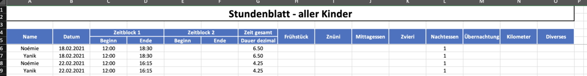
I have a sheet1 build up like structured in such a way that the name is in column A, the date in column B and the calculated total time in column G. There are more than a hundred lines of it. The name can appear several times in column A and of course the date can also appear several times.
What only happens once, however, is that the combination of name and date can only occur once.

Example:
Max 10.10.2020 9.5
Max 11.10.2020 11
Mike 11.10.2020 8.75
Mike 10.10.2020 8.5

I now have a second worksheet, where the name is entered dynamically and also a date. Now I have to find the exact combination from sheet 1, and it has to be written to me in sheet 2.

How can I do something like that - I lack any logic, because with VLOOKUP I can only use one variable.
Is it possible to run VLOOKUP or something similar until the name and then the appropriate date are found?

Thanks and regards, Mario.

 

[MarioMagnus]

Hi Dante,
this could be the problem... let me explain.
I have all the dates from a specific month in cell A20 to A50 (max. 31 days).
I have in Cell F6 the corresponding name where I need to find all the values for this name in the sheet "Zeiten". IFERROR I'm using because for the option, that no value is available for a day.
I will try your formula and give you feedback as soon as possible.
Thanks, Mario.

 

[MarioMagnus]

Hi Dante,

thanks... the formula works exact what I want. Thank you very much.
Regards, Mario.

 

[DanteAmor]

Im gald to help you, thanks for the feedback.

 

[MarioMagnus]

Hi Dante,
one more last question...
I hope you can see on the images, what I mean.

The table is build like the one image with the headers and the result will be build on the sheet2.
You can see, that for the time value that no "0" will be written when no time is available, but for each other value, when the is no source excel writes a "0" in the cell.
How can I prevent excel to write zero's in the cells where no source value is available.

Here the extended code block from you.

For y = 20 To 50
        vorlageWs.Range("B" & y).FormulaArray = "=IFERROR(INDEX(" & vTimeRng.Address(1, 1, xlA1, 1) & ",MATCH(1,(F6=" & vNameRng.Address(1, 1, xlA1, 1) & ") * (A" & y & "=" & vDateRng.Address(1, 1, xlA1, 1) & "),0)),"""")"
        vorlageWs.Range("H" & y).FormulaArray = "=IFERROR(INDEX(" & vFruehstueckRng.Address(1, 1, xlA1, 1) & ",MATCH(1,(F6=" & vNameRng.Address(1, 1, xlA1, 1) & ") * (A" & y & "=" & vDateRng.Address(1, 1, xlA1, 1) & "),0)),"""")"
        vorlageWs.Range("K" & y).FormulaArray = "=IFERROR(INDEX(" & vZnueniRng.Address(1, 1, xlA1, 1) & ",MATCH(1,(F6=" & vNameRng.Address(1, 1, xlA1, 1) & ") * (A" & y & "=" & vDateRng.Address(1, 1, xlA1, 1) & "),0)),"""")"
        vorlageWs.Range("N" & y).FormulaArray = "=IFERROR(INDEX(" & vMittagessenRng.Address(1, 1, xlA1, 1) & ",MATCH(1,(F6=" & vNameRng.Address(1, 1, xlA1, 1) & ") * (A" & y & "=" & vDateRng.Address(1, 1, xlA1, 1) & "),0)),"""")"
        vorlageWs.Range("Q" & y).FormulaArray = "=IFERROR(INDEX(" & vZvieriRng.Address(1, 1, xlA1, 1) & ",MATCH(1,(F6=" & vNameRng.Address(1, 1, xlA1, 1) & ") * (A" & y & "=" & vDateRng.Address(1, 1, xlA1, 1) & "),0)),"""")"
        vorlageWs.Range("T" & y).FormulaArray = "=IFERROR(INDEX(" & vNachtessenRng.Address(1, 1, xlA1, 1) & ",MATCH(1,(F6=" & vNameRng.Address(1, 1, xlA1, 1) & ") * (A" & y & "=" & vDateRng.Address(1, 1, xlA1, 1) & "),0)),"""")"
        vorlageWs.Range("W" & y).FormulaArray = "=IFERROR(INDEX(" & vUebernachtungRng.Address(1, 1, xlA1, 1) & ",MATCH(1,(F6=" & vNameRng.Address(1, 1, xlA1, 1) & ") * (A" & y & "=" & vDateRng.Address(1, 1, xlA1, 1) & "),0)),"""")"
        vorlageWs.Range("Z" & y).FormulaArray = "=IFERROR(INDEX(" & vKilometerRng.Address(1, 1, xlA1, 1) & ",MATCH(1,(F6=" & vNameRng.Address(1, 1, xlA1, 1) & ") * (A" & y & "=" & vDateRng.Address(1, 1, xlA1, 1) & "),0)),"""")"
        vorlageWs.Range("AA" & y).FormulaArray = "=IFERROR(INDEX(" & vDiversesRng.Address(1, 1, xlA1, 1) & ",MATCH(1,(F6=" & vNameRng.Address(1, 1, xlA1, 1) & ") * (A" & y & "=" & vDateRng.Address(1, 1, xlA1, 1) & "),0)),"""")"
    Next y

Thanks, Mario.

 

[DanteAmor]

Check this:

Display or hide zero values - Microsoft Support

Hide or display zero values in Excel worksheets by using an option in the Advanced tab, or by using a number format, using a conditional format, a function, and by hiding zeros in PivotTable reports.

support.microsoft.com

 

[MarioMagnus]

Thanks Dante...

 

[DanteAmor]

Again with pleasure. Thanks for the feedback