VBA to input ="=" into a cell?

[RockandGrohl]

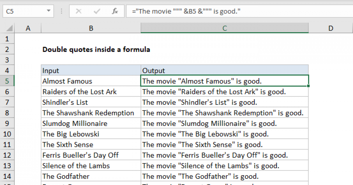
The inclusion of multiple equals and quote marks is breaking VBA's little brain - and mine!

Have tried this:

Range(Cells(2, "Q"), Cells(x, "Q")).Value = "=" & """ & " = " & """

To no luck, it just displays false.

I want the end result in the cell to be exactly:

="="

Which would then be displayed as "="

Thanks!

 

[RockandGrohl]

Hm.

Turns out if I just use "=" it works to exclude blanks from an advanced filter. Sorry for the spam!

 

[Fluff]

How about

   ActiveCell.Formula = "=""""""="""""""

 

[RockandGrohl]

How about

   ActiveCell.Formula = "=""""""="""""""

Gesundheit.

 

[Joe4]

I got it to work with a few less ", i.e.

Range(Cells(2, "Q"), Cells(x, "Q")).FormulaR1C1 = "=""="""

Note that in situations like these, let Excel do the work for you!
Simply turn on your Macro Recorder, and manually enter one of the formulas in any cell, then stop the Recorder and view the code.
That will give you exactly what you need the formula to look like in VBA!

 

[RockandGrohl]

How about

   ActiveCell.Formula = "=""""""="""""""

I got it to work with a few less ", i.e.

Range(Cells(2, "Q"), Cells(x, "Q")).FormulaR1C1 = "=""="""

Note that in situations like these, let Excel do the work for you!
Simply turn on your Macro Recorder, and manually enter one of the formulas in any cell, then stop the Recorder and view the code.
That will give you exactly what you need the formula to look like in VBA!

Hi guys, similar problem.

Cells(ActiveCell.Row, "S").FormulaR1C1 = "=SUMPRODUCT(SUBTOTAL(3,OFFSET(DataFeed!R2C35:R" & LastrowDF & "C35,ROW(DataFeed!R2C35:R" & LastrowDF & "C35)-MIN(ROW(DataFeed!R2C35:R" & LastrowDF & "C35)),,1))*[B](DataFeed!R2C35:R" & LastrowDF & "C35=""FamilyFun""))[/B]"

That last bolded part, the final bracket. What do I do if I want to swap ""FamilyFun"" out for the result of a cell on the same row in column R?

If I put in

Cells(ActiveCell.Row, "S").FormulaR1C1 = "=SUMPRODUCT(SUBTOTAL(3,OFFSET(DataFeed!R2C35:R" & LastrowDF & "C35,ROW(DataFeed!R2C35:R" & LastrowDF & "C35)-MIN(ROW(DataFeed!R2C35:R" & LastrowDF & "C35)),,1))*[B](DataFeed!R2C35:R" & LastrowDF & "C35=" & cells(activecell.row, "R").value & "))[/B]"

Then it gives me FamilyFun

But I need "FamilyFun"

Thanks!

 

[Fluff]

Maybe

"C35=""" & Cells(ActiveCell.Row, "R").Value & """))"

 

[RockandGrohl]

Maybe

"C35=""" & Cells(ActiveCell.Row, "R").Value & """))"

Perfetto. Many thanks as usual mate.

I was mucking around with double and triple quotes as per here:

Double quotes inside a formula

To include double quotes inside a formula, you can use additional double quotes. In the example shown, the formula in C5 is: ="The movie """ &B5 &""" is good."

exceljet.net

Just couldn't hack it out.

 

[Joe4]

NOTE: Going back to the original, I think I misunderstood and see that it looks like you probably wanted:
"=" with the quotes and not just =
which explains why Fluff's solution has the extra quotes!

Sorry for the misunderstanding!
But you can still follow the advice I gave, which tells you how you can come up with the solution yourself, by using the Macro Recorder.

 

[RockandGrohl]

Maybe

"C35=""" & Cells(ActiveCell.Row, "R").Value & """))"

Right, Fluff, a Mars Bar delivered straight to your gob if you can work this one out.

Brochure_Region

OptIn_NH_LandMail

Last_Booked

Last_Booked

FamilyFun

FamilyFun

UK

UK

Sports

Sports

Events

Events

EU

EU

Showtime

Showtime

OptIn_ThirdParty

OptIn_DirectEmail

Results

<>0

<>0

>=0

<=1000000

>=1

<=10000

<>0

<>0

>=0

<=1000000

>=1

<=10000

<>0

<>0

>=0

<=1000000

>=1

<=10000

In the previous formula, I helpfully had the name of the criteria in the "OptIn_DirectEmail" column (Column R)

That doesn't exist in the above table.

In the final column, Results, for each row, I need to have the same long formula as above, but in that last bracket it needs to find the name of the column header where the row isn't blank.

For example, in row 2 the formula should be

Cells(ActiveCell.Row, "S").FormulaR1C1 = "=SUMPRODUCT(SUBTOTAL(3,OFFSET(DataFeed!R2C35:R" & LastrowDF & "C35,ROW(DataFeed!R2C35:R" & LastrowDF & "C35)-MIN(ROW(DataFeed!R2C35:R" & LastrowDF & "C35)),,1))*(DataFeed!R2C35:R" & LastrowDF & "C35=""FamilyFun""))"

But instead of doing that cells(activecell.row, "R").value guff, I need to see that on that row, FamilyFun has the criteria applied, so it should be FamilyFun. On the row below, it's Events, so the next formula down would have Events, and so on.

Can you think of a way to do this? Meanwhile I'll keep thinking about it, but all I can think of is doing some kind of index-match where the result is non-blank...