VLOOKUP ERROR

Lyndon CSWP

New Member
Joined
Oct 8, 2023
Messages
10
Office Version
  1. 2010
Platform
  1. Windows
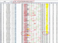
Playing around, in order to keep my mind sharp (sharp as it can get) I created a spreadsheet of Pick 3 lottery numbers and how often they have been drawn over the years. Laugh if you will. I understand they are random. However, I wanted to sort my data in an area that I could look up a 3 digit draw, sort the 6 different combinations of the 3 number and collect the data from the sheet to derive a "score" if you will, of most drawn numbers.
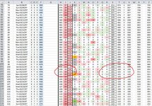
I'm using a VLOOKUP to collect a number from a column to place in the needed cell. I had got it to work but when dragging the cell down to populate the concurring cells, it did the correct thing until it got past a certain cell and failed to provide the data with a #N/A response. I cannot for the life of me figure out what I am doing wrong. I have a test spreadsheet I can supply to everyone. I'm just not sure how to attach it just yet as I finally decided to join this forum.
I'm attaching a screenshot which someone might figure out what I am referring to. If someone needs to see the actual test spreadsheet I would be glad to attach it if they can give me a clue as to how. Be gentle. I'm not likely to know what half of you would be describing as my problem with technical jargon.
 

Attachments

  • lookup issue.JPG
    lookup issue.JPG
    211.7 KB · Views: 17
Because I was trying to use a formula in which I could have 6 columns that are rearranged in different combinations of 3 digits. All I did was switch the 1, 2 ,3 in it to get these. Note the columns to the right of the column we are focusing on. I need to check these as well. The first character could be any one of the 3 digits.
 
Upvote 0

Excel Facts

Round to nearest half hour?
Use =MROUND(A2,"0:30") to round to nearest half hour. Use =CEILING(A2,"0:30") to round to next half hour.
Here I thought I was stupid or something. But the trick you showed me to test for TRUE/FALSE condition helped me to figure out what it needed to make it work. Not in any logical sense. But as it seems, the fact that I was deriving cells' data from other cells via a formula, regardless of them being formatted correctly, appears may be some sort of glitch. As you can see I have apparently figured out what I needed to do to get this to work correctly although the data in the cells were correctly formatted in the first place.
 

Attachments

  • lookup issue resolve.JPG
    lookup issue resolve.JPG
    193.6 KB · Views: 6
Upvote 0
Glad to help. Our eyes can be deceiving e.g. 100 (number) is not the same as "100" (text).
 
Upvote 0
When I evaluated the formula it showed a result as "100" but still did not derive it as a match. That is what was confusing me the most. The format showed as correct but the outcome was FALSE. The big challenge was to make text look like a number, especially when it begins with leading zeros. They are not really numbers. They are characters. This was the challenge I put forth to myself so I could learn. And even though it appeared that I was doing everything right and it showed me that I was, it still came out wrong. Do you know the simple thing I had to do to fix it? Of course, which no excel help could give me a clue? And in itself was actually kinda stupid making me think that I was stupid.
 
Upvote 0
Changing the format will not convert data that is being recognised as Text to being recognised as a number nor data being recognised as a number to being text.
In fact a quick way to check on how Excel is seeing the data is:
• Select the column
• Change the format to something that will stand out, in your case pick format as number with 2 decimal places.
• Any value that now shows 2 decimals is being recognised as a number. Anything that is being recognised as text will not change format, when you change the number format
• Ctrl+Z to undo

Ideally you want to clean up your data eg since your data is all numbers change your formula to
Excel Formula:
=VALUE(MID($S102,1,1)&MID($S102,2,1)&MID($S102,3,1))

The lookup below should mask the issues of having inconsistent data types and get you a result.
Excel Formula:
=IFERROR(VLOOKUP(TEXT(T101,"000"),$H$2:$J$1001,3,FALSE),VLOOKUP(VALUE(T101),$H$2:$J$1001,3,FALSE))
That is what I thought I needed to do in the first place was to alter my vlookup in a way that it would only look it up as text. All I did was re-enter the data in 2 of my columns with cells that I pre-formatted as text, then auto-fill the columns and that fixed it. I had no idea that changing the format after data already existed did not change the existing data format itself. Like I said. I have no idea what I'm doing, but I'm doing it.
 
Upvote 0
Solution
Don't worry you are not alone. It comes up regularly and often relating to dates (which when recognised as dates are in fact numbers in Excel).
 
Upvote 0
Well... it is what it is. And yes, I am aware of dates as well. However, I believe that this issue is resolved and I believe I have the responsibility to mark it as so. I see a check mark in an incoming message but I do not see one in this outgoing message. (Which is kinda weird to me.) But if either of the two of you that has offered their help can check it for me, I appreciate it. Otherwise I will just check a reply. Thanks much for you guys' help.
 
Upvote 0
but I do not see one in this outgoing message.
Presumably that was because you were looking at the message before you actually 'posted' it.
In any case, post #19 should not have the 'Mark as solution' checked since it does not contain the solution to your question (It is not a check mark to close the thread or indicate that no further help is required.)

To help future readers, you should mark the actual post that best answered your question.
 
Upvote 0

Forum statistics

Threads
1,215,069
Messages
6,122,954
Members
449,095
Latest member
nmaske

We've detected that you are using an adblocker.

We have a great community of people providing Excel help here, but the hosting costs are enormous. You can help keep this site running by allowing ads on MrExcel.com.
Allow Ads at MrExcel

Which adblocker are you using?

Disable AdBlock

Follow these easy steps to disable AdBlock

1)Click on the icon in the browser’s toolbar.
2)Click on the icon in the browser’s toolbar.
2)Click on the "Pause on this site" option.
Go back

Disable AdBlock Plus

Follow these easy steps to disable AdBlock Plus

1)Click on the icon in the browser’s toolbar.
2)Click on the toggle to disable it for "mrexcel.com".
Go back

Disable uBlock Origin

Follow these easy steps to disable uBlock Origin

1)Click on the icon in the browser’s toolbar.
2)Click on the "Power" button.
3)Click on the "Refresh" button.
Go back

Disable uBlock

Follow these easy steps to disable uBlock

1)Click on the icon in the browser’s toolbar.
2)Click on the "Power" button.
3)Click on the "Refresh" button.
Go back
Back
Top