VLOOKUP & MIN date

[LEXCERM]

Hi,

I would like a formula to:-

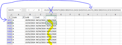
a) Find the MIN value in ColB which corresponds to value "A" in ColA (which will be 01-Feb)
b) Return the corresponding value in ColC (which will be 15-Feb)

Bearing in mind I have hundreds of rows with similar data but different values in ColA.

ColA	ColB	ColC
A	03-Feb​	01-Feb​
A	05-Feb​	08-Feb​
A	01-Feb​	15-Feb​

Also, if ColA was the last column, can this be achieved by using INDEX/MATCH etc?

Many thanks in advance.

 

[Joe4]

Here is one way. Assuming that your data is in the range A2:C4:

=XLOOKUP(MINIFS(B2:B4,A2:A4,"A"),B2:B4,C2:C4)

 

[LEXCERM]

Here is one way. Assuming that your data is in the range A2:C4:

=XLOOKUP(MINIFS(B2:B4,A2:A4,"A"),B2:B4,C2:C4)

Many thanks @Joe4 for this. I have one question. It works fine for that small example, however, when I add around 10,000 rows of data (and I have extended the range in the formula etc), the results don't match at all. Are there any limitations to this? I've tried using $ to keep the range in tact and other methods, but not quite getting the desired result. Thanks again.

 

[Joe4]

Many thanks @Joe4 for this. I have one question. It works fine for that small example, however, when I add around 10,000 rows of data (and I have extended the range in the formula etc), the results don't match at all. Are there any limitations to this? I've tried using $ to keep the range in tact and other methods, but not quite getting the desired result. Thanks again.

Sounds like you may not be doing something correctly with the formula, or may have a data issue (multiple records with the same date).

The formula, locked-down, should look something like this:

=XLOOKUP(MINIFS($B$2:$B$4,$A$2:$A$4,"A"),$B$2:$B$4,$C$2:$C$4)

But are you hard-coding in the "A" part, or using a cell reference?
If using a cell reference, that one should NOT be locked down.

 

[LEXCERM]

Sounds like you may not be doing something correctly with the formula, or may have a data issue (multiple records with the same date).

The formula, locked-down, should look something like this:

=XLOOKUP(MINIFS($B$2:$B$4,$A$2:$A$4,"A"),$B$2:$B$4,$C$2:$C$4)

But are you hard-coding in the "A" part, or using a cell reference?
If using a cell reference, that one should NOT be locked down.

I have pretty much tried all those. Here is what I have found (and the results are the same without filtering). This is the result after applying the filter:-

The date in ColD does not exist in the dataset.

However, if I apply the resized range around that dataset, I get the correct results:-

Hence why I asked about limitations.

Or maybe I'm missing something glaringly obvious lol!

Many thanks.

 

[Joe4]

Do you have the calculation mode set to manual?
It seems odd to me that all the values in column D have the same answer. That often indicates calculation mode is set to manual.
If you hit the F9 key (calculate), does it change the values?

 

[LEXCERM]

Do you have the calculation mode set to manual?
It seems odd to me that all the values in column D have the same answer. That often indicates calculation mode is set to manual.
If you hit the F9 key (calculate), does it change the values?

Calculation is set to Auto. ColD values are fine. It's looked up ColB for the min date (which is 20/9/2023), then returns the date which corresponds in ColC (4/12/2023). And this is for the values "A".

 

[Joe4]

OK, I see why. In the XLOOKUP part, we need to add the criteria to match to cell A4370 there also. Otherwise, we if other values for column A have the same date value for what we found with MINIFS, it could erroneously return those.

Try this:

=XLOOKUP(1,($B$2:$B$25522=MINIFS($B$2:$B$25522,$A$2:$A$25522,A4370))*($A$2:$A$25522=A4370),$C$2:$C$25522)

 

[LEXCERM]

OK, I see why. In the XLOOKUP part, we need to add the criteria to match to cell A4370 there also. Otherwise, we if other values for column A have the same date value for what we found with MINIFS, it could erroneously return those.

Try this:

=XLOOKUP(1,($B$2:$B$25522=MINIFS($B$2:$B$25522,$A$2:$A$25522,A4370))*($A$2:$A$25522=A4370),$C$2:$C$25522)

I shall try this soon and get back to you, but thank you so much for the help. Much appreciated.

 

[Joe4]

You are welcome!