vlookup (or index match) using multiple criteria

[vkorla]

Hello!

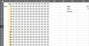
Given 2 input values, one for "Age" and the other for "Raw", how can I return the corresponding correct value?

For example, for the "Age" of 21 (cell CB2), and "Raw" of 7 (CB3), the value I want returned is 23 (cell G9).

Is this possible using xlookup?

Thank you!

 

[awoohaw]

try

Book1
	A	B	C	D	E	F	G	H	I	J	K	L	M	N	O	P	Q	R
1		Age	17	18	19	20	21	22	23	24	25	26	27	28	29
2	Raw	0	20	20	20	20	20	20	20	20	20	20	20	20	20		Age	21
3		1	20	20	20	20	20	20	20	20	20	20	20	20	20		Raw	7
4		2	20	20	20	20	20	20	20	20	20	20	20	20	20		Result	23
5		3	20	20	20	20	20	20	20	20	20	20	20	20	20
6		4	20	20	20	20	20	20	20	20	20	20	20	20	20
7		5	21	21	21	21	21	21	21	21	21	21	21	21	21
8		6	22	22	22	22	22	22	22	22	22	22	22	22	22
9		7	23	23	23	23	23	23	23	23	23	23	23	23	23
10		8	24	24	24	24	24	24	24	24	24	24	24	24	24
11		9	25	25	25	25	25	25	25	25	25	25	25	25	25
12		10	26	26	26	26	26	26	26	26	26	26	26	26	26
13		11	27	27	27	27	27	27	27	27	27	27	27	27	27
14		12	28	28	28	28	28	28	28	28	28	28	28	28	28
15		13	29	29	29	29	29	29	29	29	29	29	29	29	29
16		14	30	30	30	30	30	30	30	30	30	30	30	30	30
17		15	31	31	31	31	31	31	31	31	31	31	31	31	31
Sheet5

Cell Formulas
Range	Formula
R4	R4	=INDEX($C$2:$O$17, MATCH(R3,B2:B17,0),MATCH(R2,C1:O1))

 

[DanteAmor]

Try:

varios 10ene2024.xlsm
	A	B	C	D	E	F	G	H	I	J	K	L	M	N	O	P																																																														BZ	CA	CB
1		Age	17	18	19	20	21	22	23	24	25	26	27	28	29
2	Raw	0	20	29	30	28	20	28	21	25	20	23	27	22	28																																																																Age	21
3		1	23	29	30	24	22	21	31	28	31	30	26	20	23																																																																Raw	7
4		2	23	23	25	29	27	21	28	28	26	31	23	23	25																																																																Result	77
5		3	23	26	29	24	26	21	24	24	31	23	21	31	20
6		4	23	26	23	24	26	23	25	21	22	26	30	27	25
7		5	24	27	30	21	24	29	26	20	26	31	24	31	26
8		6	29	30	20	22	27	27	24	28	29	27	24	24	23
9		7	25	26	21	27	77	23	25	24	27	23	24	31	28
10		8	20	21	24	25	25	27	20	20	31	31	30	27	26
11		9	21	28	20	20	29	30	21	25	30	26	29	22	21
12		10	30	26	23	22	30	31	31	26	30	25	31	23	28
13		11	22	24	27	29	23	31	26	29	26	28	26	21	20
14		12	28	28	27	24	21	20	20	22	23	30	26	26	24
15		13	26	22	21	21	27	21	22	24	28	30	25	22	23
16		14	29	22	24	23	25	20	25	20	20	25	28	30	27
17		15	20	27	30	25	25	26	28	27	25	22	21	31	88
Hoja5

Cell Formulas
Range	Formula
CB4	CB4	=INDEX(C2:O17,MATCH(CB3,B2:B17,0),MATCH(CB2,C1:O1,0))

 

[vkorla]

Ah, thanks so much @DanteAmor! For the MATCH part I was doing match(CB3=B2:B17)*(CB2=C1:O1) ... for some weird reason.

 

[DanteAmor]

For the MATCH part I was doing match(CB3=B2:B17)*(CB2=C1:O1) ... for some weird reason.

For that it should be with the SumProduct function, but it works only with numbers in the array:

varios 10ene2024.xlsm
	A	B	C	D	E	F	G	H	I	J	K	L	M	N	O	P																																																														BZ	CA	CB
1		Age	17	18	19	20	21	22	23	24	25	26	27	28	29
2	Raw	0	20	29	30	28	20	28	21	25	20	23	27	22	28																																																																Age	21
3		1	23	29	30	24	22	21	31	28	31	30	26	20	23																																																																Raw	7
4		2	23	23	25	29	27	21	28	28	26	31	23	23	25																																																																Result	77
5		3	23	26	29	24	26	21	24	24	31	23	21	31	20
6		4	23	26	23	24	26	23	25	21	22	26	30	27	25
7		5	24	27	30	21	24	29	26	20	26	31	24	31	26
8		6	29	30	20	22	27	27	24	28	29	27	24	24	23
9		7	25	26	21	27	77	23	25	24	27	23	24	31	28
10		8	20	21	24	25	25	27	20	20	31	31	30	27	26
11		9	21	28	20	20	29	30	21	25	30	26	29	22	21
12		10	30	26	23	22	30	31	31	26	30	25	31	23	28
13		11	22	24	27	29	23	31	26	29	26	28	26	21	20
14		12	28	28	27	24	21	20	20	22	23	30	26	26	24
15		13	26	22	21	21	27	21	22	24	28	30	25	22	23
16		14	29	22	24	23	25	20	25	20	20	25	28	30	27
17		15	20	27	30	25	25	26	28	27	25	22	21	31	88
18
Hoja5

Cell Formulas
Range	Formula
CB4	CB4	=SUMPRODUCT((B2:B17=CB3)*(C1:O1=CB2)*(C2:O17))

 

[vkorla]

try

Book1
	A	B	C	D	E	F	G	H	I	J	K	L	M	N	O	P	Q	R
1		Age	17	18	19	20	21	22	23	24	25	26	27	28	29
2	Raw	0	20	20	20	20	20	20	20	20	20	20	20	20	20		Age	21
3		1	20	20	20	20	20	20	20	20	20	20	20	20	20		Raw	7
4		2	20	20	20	20	20	20	20	20	20	20	20	20	20		Result	23
5		3	20	20	20	20	20	20	20	20	20	20	20	20	20
6		4	20	20	20	20	20	20	20	20	20	20	20	20	20
7		5	21	21	21	21	21	21	21	21	21	21	21	21	21
8		6	22	22	22	22	22	22	22	22	22	22	22	22	22
9		7	23	23	23	23	23	23	23	23	23	23	23	23	23
10		8	24	24	24	24	24	24	24	24	24	24	24	24	24
11		9	25	25	25	25	25	25	25	25	25	25	25	25	25
12		10	26	26	26	26	26	26	26	26	26	26	26	26	26
13		11	27	27	27	27	27	27	27	27	27	27	27	27	27
14		12	28	28	28	28	28	28	28	28	28	28	28	28	28
15		13	29	29	29	29	29	29	29	29	29	29	29	29	29
16		14	30	30	30	30	30	30	30	30	30	30	30	30	30
17		15	31	31	31	31	31	31	31	31	31	31	31	31	31
Sheet5

Cell Formulas
Range	Formula
R4	R4	=INDEX($C$2:$O$17, MATCH(R3,B2:B17,0),MATCH(R2,C1:O1))

thank you @awoohaw

 

[awoohaw]

You're welcome. My solution was nearly the same as @DanteAmor 's but I didn't go to the trouble of using the exact same column references as you requested, and I did miss a zero in the 2nd match function.

Best Wishes!