Vlookup result changing after adding iferror

[lizmorton1990]

Hi,

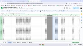
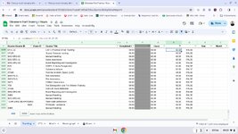
I am trying to do a vlookup and I want to add an iferror in if the vlookup doesn't find anything so it looks at another cell. So far I started with this:

=vlookup(C11194,Hours!A:AC,29,0)

Which returned 08:00 to mean 8 hours of training but when that returns an error as the data doesn't exist, I want to add an iferror to the vlookup so when it says #n/a it looks at another cells on the same tab the vlookup is on i.e

=iferror(vlookup(C11194,Hours!A:AC,29,0),M11194)

But when I do it now returns 0.3333333333 which is incorrect as it should return 08:00 in this example. For the rows that return #n/a it returns the value correctly in column M

What am I doing wrong? I have tried formatting the column to auto and plain text and it doesn't help.

 

[SunnyAlv]

Try

=TEXT(iferror(vlookup(C11194,Hours!A:AC,29,0),M11194),"h:mm")

 

[arthurbr]

0.3333333 is the underlying values of 08:00 as XL considers a day (or 24hrs) to be 1, so 8 hours =8/24 = 0.33333..Formatting as time helps

 

[lizmorton1990]

Thank-you, that has taken the 0.3333 away but some rows don't display the right information. I basically want to create a pivot that sums up column O for the number of training hours. Here's some screenshots of my data, I did try formatting to time which works and removes the 0.3333 and converts it to the actual minutes and hours but the pivot then doesn't show a sum of the hours, even when I highlight column O it shows 7 hours which isn't right considering each row is worth 5 hours.

 

[Peter_SSs]

Is this a Google Sheets question or a Microsoft Excel question?

 

[lizmorton1990]

I am using google sheets to do this one, but I didn't think formula's differed between excel and google, let me know if I am posting in the wrong place.

 

[Peter_SSs]

let me know if I am posting in the wrong place.

Yes you are ..

.. so I have moved your thread to the appropriate forum.

 

[lizmorton1990]

Thank-you

 

[Alex Blakenburg]

Try formatting your pivot values as [hh]:mm

 

[lizmorton1990]

That's worked thank-you!!! Something simple as well, oh well learnt something today