Vlookup Returning Duplicate Values

[IrisDiane]

Hello! I'm having some trouble with Vlookup (I'm quite new to Excel)

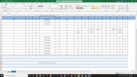
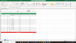
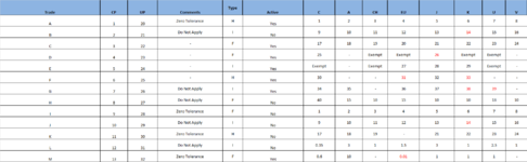
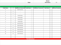
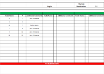
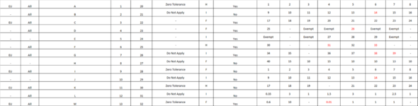
I'm trying to produce a report that returns rows that contain the word "EU" in the first column. However when a row is blank, it gives me multiple values for the next cell it finds the word "EU" in. Any help would be greatly appreciated!

 

[Saurabhj]

Hi IrisDiane,

The screenshots Ist Sheet is not clear. Also in your case Vlookup will not work.

Please share the screenshot again and the expected result.

Thanks,
Saurabh

 

[IrisDiane]

Thanks for the reply, here's the updated pictures (Hopefully they came out okay)

 

[Saurabhj]

Hi,
Thanks for sharing the clear images.

You are checking "EU" in A5 to C17 cells but in Picture1 the first column doesn't contain EU and thus unable to understand how Wanted Results you received.

Please explain the criteria you are using to get the result.

Thanks,
Saurabh

 

[IrisDiane]

Apologies once again, I didn't get the full image.

 

[Peter_SSs]

Images are difficult anyway as we cannot copy from them. A better option is:

MrExcel has a tool called “XL2BB” that lets you post samples of your data that will allow us to copy/paste it to our Excel spreadsheets, so we can work with the same copy of data that you are. Instructions on using this tool can be found here: XL2BB Add-in

Note that there is also a "Test Here” forum on this board. This is a place where you can test using this tool (or any other posting techniques that you want to test) before trying to use those tools in your actual posts.

 

[IrisDiane]

Copy.xlsx
	A	B	C	D	E	F	G	H	I	J	K	L	M	N	O	P
4	EU	All	Trade	CP	UP	Comments	Type	Active	C	A	CH	EU	J	K	U	V
5	EU	All	A	1	20	Zero Tolerance	H	Yes	1	2	3	4	5	6	7	8
6	-	All	B	2	21	Do Not Apply	I	No	9	10	11	12	13	14	15	16
7	EU	All	C	3	22	-	F	Yes	17	18	19	20	21	22	23	24
8	-	All	D	4	23	-	F	Yes	25	-	Exempt	Exempt	26	Exempt	Exempt	-
9	-	-	E	5	24	-	I	Yes	Exempt	-	Exempt	27	28	29	Exempt	-
10	-	All	F	6	25	-	H	Yes	30	-	-	31	32	33	-	-
11	EU	All	G	7	26	Do Not Apply	I	Yes	34	35	-	36	37	38	39	-
12	-	-	H	8	27	Do Not Apply	F	No	40	15	10	15	10	10	13	10
13	EU	All	I	9	28	Zero Tolerance	F	No	1	2	3	4	5	6	7	8
14	-	-	J	10	29	Do Not Apply	I	No	9	10	11	12	13	14	15	16
15	EU	All	K	11	30	Zero Tolerance	H	No	17	18	19	-	21	22	23	24
16	-	All	L	12	31	Do Not Apply	I	No	0.35	3	1	1.5	3	1	2.5	1
17	EU	All	M	13	32	Zero Tolerance	F	Yes	0.6	10	-	0.01	1	1	1	-
18
19
20
21
22
23
24
25
26
Blue

Copy.xlsx
	A	B	C	D	E	F	G	H	I
1
2				Orgin:			Market Destination:		EU
3
4
5
6
7	Trade Name	P	Additional Comments	Trade Name		Additional Comments	Trade Name		Additional Comments
8	A	1	Zero Tolerance
9	C	3	-
10	C	3	-
11	G	7	Do Not Apply
12	G	7	Do Not Apply
13	G	7	Do Not Apply
14	G	7	Do Not Apply
15	I	9	Zero Tolerance
16	I	9	Zero Tolerance
17	K	11	Zero Tolerance
18	K	11	Zero Tolerance
19	M	13	Zero Tolerance
20	M	13	Zero Tolerance
21
22
23	No Substitutions
24
25
26
27
Blue EU

Cell Formulas
Range	Formula
A8:A20	A8	=VLOOKUP(I$2,'Blue '!A5:C$17,3,FALSE)
B8:B20	B8	=VLOOKUP(I$2,'Blue '!A5:D$17,4,FALSE)
C8:C20	C8	=VLOOKUP(I$2,'Blue '!A5:F$17,6,FALSE)

Cells with Data Validation
Cell	Allow	Criteria
F2:F3	List	=#REF!
C2:C3	List	=#REF!

Copy.xlsx
	A	B	C	D	E	F	G	H	I
1
2				Orgin:			Market Destination:		EU
3
4
5
6
7	Trade Name	P	Additional Comments	Trade Name		Additional Comments	Trade Name		Additional Comments
8	A	1	Zero Tolerance
9	C	3	-
10	G	7	Do Not Apply
11	I	9	Zero Tolerance
12	K	11	Zero Tolerance
13	M	13	Zero Tolerance
14
15
16
17
18
19
20
21
22	No Substitutions
23
24
25
26
Wanted Result

Cell Formulas
Range	Formula
A8:A9	A8	=VLOOKUP(I$2,'Blue '!A5:C$17,3,FALSE)
B8:B9	B8	=VLOOKUP(I$2,'Blue '!A5:D$17,4,FALSE)
C8:C9	C8	=VLOOKUP(I$2,'Blue '!A5:F$17,6,FALSE)
A10	A10	=VLOOKUP(I$2,'Blue '!A8:C$17,3,FALSE)
B10	B10	=VLOOKUP(I$2,'Blue '!A8:D$17,4,FALSE)
C10	C10	=VLOOKUP(I$2,'Blue '!A8:F$17,6,FALSE)
A11	A11	=VLOOKUP(I$2,'Blue '!A12:C$17,3,FALSE)
B11	B11	=VLOOKUP(I$2,'Blue '!A12:D$17,4,FALSE)
C11	C11	=VLOOKUP(I$2,'Blue '!A12:F$17,6,FALSE)
A12	A12	=VLOOKUP(I$2,'Blue '!A14:C$17,3,FALSE)
B12	B12	=VLOOKUP(I$2,'Blue '!A14:D$17,4,FALSE)
C12	C12	=VLOOKUP(I$2,'Blue '!A14:F$17,6,FALSE)
A13	A13	=VLOOKUP(I$2,'Blue '!A16:C$17,3,FALSE)
B13	B13	=VLOOKUP(I$2,'Blue '!A16:D$17,4,FALSE)
C13	C13	=VLOOKUP(I$2,'Blue '!A16:F$17,6,FALSE)

Cells with Data Validation
Cell	Allow	Criteria
C2:C3	List	=#REF!
F2:F3	List	=#REF!

 

[Peter_SSs]

Thanks, XL2BB makes it much easier!!

Try these, copied down

IrisDiane.xlsm
	A	B	C	D	E	F	G	H	I
1
2				Orgin:			Market Destination:		EU
3
4
5
6
7	Trade Name	P	Additional Comments	Trade Name		Additional Comments	Trade Name		Additional Comments
8	A	1	Zero Tolerance
9	C	3	-
10	G	7	Do Not Apply
11	I	9	Zero Tolerance
12	K	11	Zero Tolerance
13	M	13	Zero Tolerance
14
15
16
Blue EU

Cell Formulas
Range	Formula
A8:A16	A8	=IFERROR(INDEX(Blue!C:C,AGGREGATE(15,6,ROW(Blue!C$5:C$17)/(Blue!A$5:A$17=I$2),ROWS(A$8:A8))),"")
B8:B16	B8	=IFERROR(INDEX(Blue!D:D,AGGREGATE(15,6,ROW(Blue!D$5:D$17)/(Blue!A$5:A$17=I$2),ROWS(B$8:B8))),"")
C8:C16	C8	=IFERROR(INDEX(Blue!F:F,AGGREGATE(15,6,ROW(Blue!F$5:F$17)/(Blue!A$5:A$17=I$2),ROWS(C$8:C8))),"")

 

[IrisDiane]

Wonderful! Thank you

 

[Peter_SSs]

You're welcome. Thanks for the follow-up.