Vlookup

[ifu06416]

Hi there,

I'm looking to set up a Vlookup formula to pull through the whole numbers from a list base on what category they belong to.

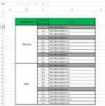
So in column F if i wanted the whole numbers associated with the planning category it would return 1, 2 & 3. If i wanted the numbers associated with PMO it would read 4 & 5. Each number would have it own cell.

Does anyone have any thoughts.

regards,

john,

 

[Eric W]

The biggest problem with your layout is the merged cells. It's very difficult to recognize that all the rows from 4 to 14 are Planning rows. You can unmerge B4:B14 and put Planning in each of them, or you can add a helper column as I did in column E. You can hide it if you don't want to see it. The G4 formula is for versions of Excel with FILTER, the F4 formula is for earlier versions. It would help if you could update your profile with the version you're using.

Book1 (version 1).xlsb
	A	B	C	D	E	F	G
1
2
3		Workstream	Outline Number	Task		PMO
4		Planning	1		Planning	4	4
5			1.1		Planning	5	5
6			1.2		Planning
7			2		Planning
8			2.1		Planning
9			2.2		Planning
10			2.3		Planning
11			2.4		Planning
12			3		Planning
13			3.1		Planning
14			3.3		Planning
15		PMO	4		PMO
16			4.1		PMO
17			4.2		PMO
18			4.3		PMO
19			4.4		PMO
20			4.5		PMO
21			4.6		PMO
22			5		PMO
23			5.1		PMO
24			5.2		PMO
25			5.2.3		PMO
26			5.3		PMO
Sheet12

Cell Formulas
Range	Formula
G4:G5	G4	=FILTER(C4:C26,(E4:E26=F3)*IFERROR(INT(C4:C26)=C4:C26,0))
F4:F10	F4	=IFERROR(AGGREGATE(15,6,$C$4:$C$26/(INT($C$4:$C$26)=$C$4:$C$26)/($E$4:$E$26=$F$3),ROWS($F$4:$F4)),"")
E4:E26	E4	=IF(B4<>"",B4,E3)
Dynamic array formulas.

 

[ifu06416]

The biggest problem with your layout is the merged cells. It's very difficult to recognize that all the rows from 4 to 14 are Planning rows. You can unmerge B4:B14 and put Planning in each of them, or you can add a helper column as I did in column E. You can hide it if you don't want to see it. The G4 formula is for versions of Excel with FILTER, the F4 formula is for earlier versions. It would help if you could update your profile with the version you're using.

Book1 (version 1).xlsb
	A	B	C	D	E	F	G
1
2
3		Workstream	Outline Number	Task		PMO
4		Planning	1		Planning	4	4
5			1.1		Planning	5	5
6			1.2		Planning
7			2		Planning
8			2.1		Planning
9			2.2		Planning
10			2.3		Planning
11			2.4		Planning
12			3		Planning
13			3.1		Planning
14			3.3		Planning
15		PMO	4		PMO
16			4.1		PMO
17			4.2		PMO
18			4.3		PMO
19			4.4		PMO
20			4.5		PMO
21			4.6		PMO
22			5		PMO
23			5.1		PMO
24			5.2		PMO
25			5.2.3		PMO
26			5.3		PMO
Sheet12

Cell Formulas
Range	Formula
G4:G5	G4	=FILTER(C4:C26,(E4:E26=F3)*IFERROR(INT(C4:C26)=C4:C26,0))
F4:F10	F4	=IFERROR(AGGREGATE(15,6,$C$4:$C$26/(INT($C$4:$C$26)=$C$4:$C$26)/($E$4:$E$26=$F$3),ROWS($F$4:$F4)),"")
E4:E26	E4	=IF(B4<>"",B4,E3)
Dynamic array formulas.

Hi there,

Thanks for this! The formula was far more complicated than I could have figured out myself.

The helper column makes sense though and it all works great.

Thanks again,

John.