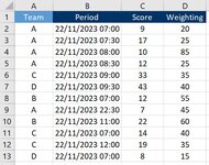
Weighted Average (Less Than - Equal To)

[dougztk]

Based on a data set I have I'm looking to calculate a weighted average for each team based on Period (ie. Team A's score up until 08:00 only).

Can this be done using a Sumproduct or is there a different/easier way to do this?

 

[AhoyNC]

If the Period will always be the same day as in your example:

Book1
	A	B	C	D	E	F	G
1	Team	Period	Score	Weighting		Team	Period
2	A	11/22/2023 7:00	9	20		A	11/22/2023 8:00
3	A	11/22/2023 7:30	17	25		40.417
4	A	11/22/2023 8:00	10	85
5	A	11/22/2023 8:30	12	25
6	c	11/22/2023 9:00	33	35
7	D	11/22/2023 9:30	43	40
8	B	11/22/2023 7:00	12	55
9	A	11/22/2023 22:30	7	45
10	B	11/22/2023 11:00	22	60
11	c	11/22/2023 7:00	14	40
12	c	11/22/2023 12:00	19	35
13	D	11/22/2023 7:00	8	15
Sheet2

Cell Formulas
Range	Formula
F3	F3	=SUMPRODUCT(--($A$2:$A$13=$F$2),--($B$2:$B$13<=G2),($C$2:$C$13),$D$2:$D$13)/SUMIFS($C$2:$C$13,$A$2:$A$13,$F$2,$B$2:$B$13,"<="&$G$2)

 

[awoohaw]

this is not using the sumproduct.
And, this also only averages the items that are selected in the filter.

Book1
	A	B	C	D	E	F	G
1	TEAM	PERIOD	SCORE	Weighting		time cutoff:	08:00:00
2	A	2023-11-22 07:00	9	20
3	A	2023-11-22 07:30	17	25
4	A	2023-11-22 08:00	10	85		A	11.1923077
5	A	2023-11-22 08:30	12	25		B	12
6	C	2023-11-22 09:00	33	35		C	14
7	D	2023-11-22 09:30	43	40		D	8
8	B	2023-11-22 07:00	12	55
9	A	2023-11-22 22:30	7	45
10	B	2023-11-22 11:00	22	60
11	C	2023-11-22 07:00	14	40
12	C	2023-11-22 12:00	19	35
13	D	2023-11-22 07:00	8	15
Sheet3

Cell Formulas
Range	Formula
G4:G7	G4	=SUM((F4=$A$2:$A$13)*(ROUND(MOD($B$2:$B$13,1),10)<=$G$1)*($C$2:$C$13)*($D$2:$D$13)) / SUM((F4=$A$2:$A$13)*(ROUND(MOD($B$2:$B$13,1),10)<=$G$1)*($D$2:$D$13))

 

[dougztk]

If the Period will always be the same day as in your example:

Book1
	A	B	C	D	E	F	G
1	Team	Period	Score	Weighting		Team	Period
2	A	11/22/2023 7:00	9	20		A	11/22/2023 8:00
3	A	11/22/2023 7:30	17	25		40.417
4	A	11/22/2023 8:00	10	85
5	A	11/22/2023 8:30	12	25
6	c	11/22/2023 9:00	33	35
7	D	11/22/2023 9:30	43	40
8	B	11/22/2023 7:00	12	55
9	A	11/22/2023 22:30	7	45
10	B	11/22/2023 11:00	22	60
11	c	11/22/2023 7:00	14	40
12	c	11/22/2023 12:00	19	35
13	D	11/22/2023 7:00	8	15
Sheet2

Cell Formulas
Range	Formula
F3	F3	=SUMPRODUCT(--($A$2:$A$13=$F$2),--($B$2:$B$13<=G2),($C$2:$C$13),$D$2:$D$13)/SUMIFS($C$2:$C$13,$A$2:$A$13,$F$2,$B$2:$B$13,"<="&$G$2)

This works perfectly, thank you!

 

[AhoyNC]

You're welcome. Thanks for the feedback and welcome to the forum.