Get.cell (an old xl 4 macro function) can be used to return more info about the worksheet environment than is available with the cell() function. No VBA code (or skills) are required. One complication is that you cannot use get.cell directly in the worksheet. However, there is a work-around...
The method is as follows:
1) Determine which of the get.cell arguments you need - see the full list below.
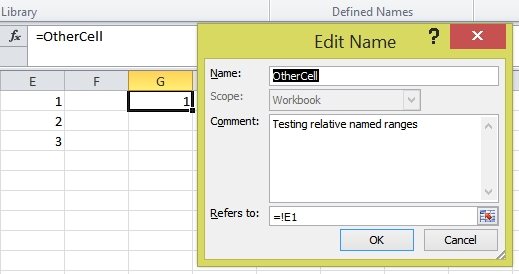
2) Go to Insert | Name | Define.
3) Type a suitably descriptive name (e.g. CellHasFormula, or CellFont etc)
5) In the refers to box, type something of the following format:
=GET.CELL(48,INDIRECT("rc",FALSE))
This will return info about the cell the final formula is in. To use get.cell to return info about cells other than the ones the formulas are in, , you will need to use on offset, e.g.:
=GET.CELL(48,OFFSET(INDIRECT("RC",FALSE),0,1))
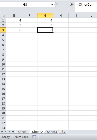
6) enter =CellHasFormula etc in the desired cells.
What follows is a full list of the get.cell arguments. The full help file for excel 4 macros is available here:
http://support.microsoft.com/default.aspx?scid=KB;EN-US;Q128185&ID=KB;EN-US;Q128185&FR=1<pre>
Returns information about the formatting, location, or contents of a cell.
Use GET.CELL in a macro whose behavior is determined by the status of a particular cell.
Syntax
GET.CELL(type_num, reference)
Type_num is a number that specifies what type of cell information you want.
The following list shows the possible values of type_num and the corresponding results.
Type_num Returns
1 Absolute reference of the upper-left cell in reference, as text in the current workspace reference style.
2 Row number of the top cell in reference.
3 Column number of the leftmost cell in reference.
4 Same as TYPE(reference).
5 Contents of reference.
6 Formula in reference, as text, in either A1 or R1C1 style depending on the workspace setting.
7 Number format of the cell, as text (for example, "m/d/yy" or "General").
8 Number indicating the cell's horizontal alignment:
15 If the cell's formula is hidden, returns TRUE; otherwise, returns FALSE.
16 A two-item horizontal array containing the width of the active cell and a logical value
18 Name of font, as text.
19 Size of font, in points.
20 If all the characters in the cell, or only the first character, are bold, returns TRUE; otherwise, returns FALSE.
21 If all the characters in the cell, or only the first character, are italic, returns TRUE; otherwise, returns FALSE.
22 If all the characters in the cell, or only the first character, are underlined, returns TRUE; otherwise, returns FALSE.
23 If all the characters in the cell, or only the first character, are struck through, returns TRUE; otherwise, returns FALSE.
24 Font color of the first character in the cell, as a number in the range 1 to 56. If font color is automatic, returns 0.
25 If all the characters in the cell, or only the first character, are outlined, returns TRUE; otherwise, returns FALSE.
29 Column level (outline).
30 If the row containing the active cell is a summary row, returns TRUE; otherwise, returns FALSE.
31 If the column containing the active cell is a summary column, returns TRUE; otherwise, returns FALSE.
32 Name of the workbook and sheet containing the cell If the window contains only a single sheet that has the same
34 Left-border color as a number in the range 1 to 56. If color is automatic, returns 0.
35 Right-border color as a number in the range 1 to 56. If color is automatic, returns 0.
36 Top-border color as a number in the range 1 to 56. If color is automatic, returns 0.
37 Bottom-border color as a number in the range 1 to 56. If color is automatic, returns 0.
38 Shade foreground color as a number in the range 1 to 56. If color is automatic, returns 0.
39 Shade background color as a number in the range 1 to 56. If color is automatic, returns 0.
40 Style of the cell, as text.
41 Returns the formula in the active cell without translating it (useful for international macro sheets).
42 The horizontal distance, measured in points, from the left edge of the active window to the left edge of the cell.
47 If the cell contains a sound note, returns TRUE; otherwise, returns FALSE.
48 If the cells contains a formula, returns TRUE; if a constant, returns FALSE.
49 If the cell is part of an array, returns TRUE; otherwise, returns FALSE.
50 Number indicating the cell's vertical alignment:
53 Contents of the cell as it is currently displayed, as text, including any additional numbers or symbols resulting from the cell's formatting.
54 Returns the name of the PivotTable view containing the active cell.
55 Returns the position of a cell within the PivotTableView.
56 Returns the name of the field containing the active cell reference if inside a PivotTable view.
57 Returns TRUE if all the characters in the cell, or only the first character, are formatted with a superscript font; otherwise, returns FALSE.
58 Returns the font style as text of all the characters in the cell, or only the first character as displayed in the Font tab of the Format Cells dialog box: for example, "Bold Italic".
59 Returns the number for the underline style:
60 Returns TRUE if all the characters in the cell, or only the first characrter, are formatted with a subscript font; otherwise, it returns FALSE.
61 Returns the name of the PivotTable item for the active cell, as text.
62 Returns the name of the workbook and the current sheet in the form "[book1]sheet1".
63 Returns the fill (background) color of the cell.
64 Returns the pattern (foreground) color of the cell.
65 Returns TRUE if the Add Indent alignment option is on (Far East versions of Microsoft Excel only); otherwise, it returns FALSE.
66 Returns the book name of the workbook containing the cell in the form BOOK1.XLS.
Reference is a cell or a range of cells from which you want information.
If reference is a range of cells, the cell in the upper-left corner of the first range in reference is used.
If reference is omitted, the active cell is assumed.
Tip Use GET.CELL(17) to determine the height of a cell and GET.CELL(44) - GET.CELL(42) to determine the width.
Examples
The following macro formula returns TRUE if cell B4 on sheet Sheet1 is bold:
GET.CELL(20, Sheet1!$B$4)
You can use the information returned by GET.CELL to initiate an action.
The following macro formula runs a custom function named BoldCell if the GET.CELL formula returns FALSE:
IF(GET.CELL(20, Sheet1!$B$4), , BoldCell())</pre>
This message was edited by PaddyD on 2002-09-05 22:02
The method is as follows:
1) Determine which of the get.cell arguments you need - see the full list below.
2) Go to Insert | Name | Define.
3) Type a suitably descriptive name (e.g. CellHasFormula, or CellFont etc)
5) In the refers to box, type something of the following format:
=GET.CELL(48,INDIRECT("rc",FALSE))
This will return info about the cell the final formula is in. To use get.cell to return info about cells other than the ones the formulas are in, , you will need to use on offset, e.g.:
=GET.CELL(48,OFFSET(INDIRECT("RC",FALSE),0,1))
6) enter =CellHasFormula etc in the desired cells.
What follows is a full list of the get.cell arguments. The full help file for excel 4 macros is available here:
http://support.microsoft.com/default.aspx?scid=KB;EN-US;Q128185&ID=KB;EN-US;Q128185&FR=1<pre>
Returns information about the formatting, location, or contents of a cell.
Use GET.CELL in a macro whose behavior is determined by the status of a particular cell.
Syntax
GET.CELL(type_num, reference)
Type_num is a number that specifies what type of cell information you want.
The following list shows the possible values of type_num and the corresponding results.
Type_num Returns
1 Absolute reference of the upper-left cell in reference, as text in the current workspace reference style.
2 Row number of the top cell in reference.
3 Column number of the leftmost cell in reference.
4 Same as TYPE(reference).
5 Contents of reference.
6 Formula in reference, as text, in either A1 or R1C1 style depending on the workspace setting.
7 Number format of the cell, as text (for example, "m/d/yy" or "General").
8 Number indicating the cell's horizontal alignment:
1 = General
2 = Left
3 = Center
4 = Right
5 = Fill
6 = Justify
7 = Center across cells
9 Number indicating the left-border style assigned to the cell:0 = No border
1 = Thin line
2 = Medium line
3 = Dashed line
4 = Dotted line
5 = Thick line
6 = Double line
7 = Hairline
10 Number indicating the right-border style assigned to the cell.See type_num 9 for descriptions of the numbers returned.
11 Number indicating the top-border style assigned to the cell.See type_num 9 for descriptions of the numbers returned.
12 Number indicating the bottom-border style assigned to the cell.See type_num 9 for descriptions of the numbers returned.
13 Number from 0 to 18, indicating the pattern of the selected cellas displayed in the Patterns tab of the Format Cells dialog box,
which appears when you choose the Cells command from the Format menu.
If no pattern is selected, returns 0.
14 If the cell is locked, returns TRUE; otherwise, returns FALSE.15 If the cell's formula is hidden, returns TRUE; otherwise, returns FALSE.
16 A two-item horizontal array containing the width of the active cell and a logical value
indicating whether the cell's width is set to change as the standard width changes (TRUE)
or is a custom width (FALSE).
17 Row height of cell, in points.18 Name of font, as text.
19 Size of font, in points.
20 If all the characters in the cell, or only the first character, are bold, returns TRUE; otherwise, returns FALSE.
21 If all the characters in the cell, or only the first character, are italic, returns TRUE; otherwise, returns FALSE.
22 If all the characters in the cell, or only the first character, are underlined, returns TRUE; otherwise, returns FALSE.
23 If all the characters in the cell, or only the first character, are struck through, returns TRUE; otherwise, returns FALSE.
24 Font color of the first character in the cell, as a number in the range 1 to 56. If font color is automatic, returns 0.
25 If all the characters in the cell, or only the first character, are outlined, returns TRUE; otherwise, returns FALSE.
Outline font format is not supported by Microsoft Excel for Windows.
26 If all the characters in the cell, or only the first character, are shadowed, returns TRUE; otherwise, returns FALSE.Shadow font format is not supported by Microsoft Excel for Windows.
27 Number indicating whether a manual page break occurs at the cell:0 = No break
1 = Row
2 = Column
3 = Both row and column
28 Row level (outline).29 Column level (outline).
30 If the row containing the active cell is a summary row, returns TRUE; otherwise, returns FALSE.
31 If the column containing the active cell is a summary column, returns TRUE; otherwise, returns FALSE.
32 Name of the workbook and sheet containing the cell If the window contains only a single sheet that has the same
name as the workbook without its extension, returns only the name of the book, in the form BOOK1.XLS.
Otherwise, returns the name of the sheet in the form "[Book1]Sheet1".
33 If the cell is formatted to wrap, returns TRUE; otherwise, returns FALSE.34 Left-border color as a number in the range 1 to 56. If color is automatic, returns 0.
35 Right-border color as a number in the range 1 to 56. If color is automatic, returns 0.
36 Top-border color as a number in the range 1 to 56. If color is automatic, returns 0.
37 Bottom-border color as a number in the range 1 to 56. If color is automatic, returns 0.
38 Shade foreground color as a number in the range 1 to 56. If color is automatic, returns 0.
39 Shade background color as a number in the range 1 to 56. If color is automatic, returns 0.
40 Style of the cell, as text.
41 Returns the formula in the active cell without translating it (useful for international macro sheets).
42 The horizontal distance, measured in points, from the left edge of the active window to the left edge of the cell.
May be a negative number if the window is scrolled beyond the cell.
43 The vertical distance, measured in points, from the top edge of the active window to the top edge of the cell.May be a negative number if the window is scrolled beyond the cell.
44 The horizontal distance, measured in points, from the left edge of the active window to the right edge of the cell.May be a negative number if the window is scrolled beyond the cell.
45 The vertical distance, measured in points, from the top edge of the active window to the bottom edge of the cell.May be a negative number if the window is scrolled beyond the cell.
46 If the cell contains a text note, returns TRUE; otherwise, returns FALSE.47 If the cell contains a sound note, returns TRUE; otherwise, returns FALSE.
48 If the cells contains a formula, returns TRUE; if a constant, returns FALSE.
49 If the cell is part of an array, returns TRUE; otherwise, returns FALSE.
50 Number indicating the cell's vertical alignment:
1 = Top
2 = Center
3 = Bottom
4 = Justified
51 Number indicating the cell's vertical orientation:0 = Horizontal
1 = Vertical
2 = Upward
3 = Downward
52 The cell prefix (or text alignment) character, or empty text ("") if the cell does not contain one.53 Contents of the cell as it is currently displayed, as text, including any additional numbers or symbols resulting from the cell's formatting.
54 Returns the name of the PivotTable view containing the active cell.
55 Returns the position of a cell within the PivotTableView.
56 Returns the name of the field containing the active cell reference if inside a PivotTable view.
57 Returns TRUE if all the characters in the cell, or only the first character, are formatted with a superscript font; otherwise, returns FALSE.
58 Returns the font style as text of all the characters in the cell, or only the first character as displayed in the Font tab of the Format Cells dialog box: for example, "Bold Italic".
59 Returns the number for the underline style:
1 = none
2 = single
3 = double
4 = single accounting
5 = double accounting
60 Returns TRUE if all the characters in the cell, or only the first characrter, are formatted with a subscript font; otherwise, it returns FALSE.
61 Returns the name of the PivotTable item for the active cell, as text.
62 Returns the name of the workbook and the current sheet in the form "[book1]sheet1".
63 Returns the fill (background) color of the cell.
64 Returns the pattern (foreground) color of the cell.
65 Returns TRUE if the Add Indent alignment option is on (Far East versions of Microsoft Excel only); otherwise, it returns FALSE.
66 Returns the book name of the workbook containing the cell in the form BOOK1.XLS.
Reference is a cell or a range of cells from which you want information.
If reference is a range of cells, the cell in the upper-left corner of the first range in reference is used.
If reference is omitted, the active cell is assumed.
Tip Use GET.CELL(17) to determine the height of a cell and GET.CELL(44) - GET.CELL(42) to determine the width.
Examples
The following macro formula returns TRUE if cell B4 on sheet Sheet1 is bold:
GET.CELL(20, Sheet1!$B$4)
You can use the information returned by GET.CELL to initiate an action.
The following macro formula runs a custom function named BoldCell if the GET.CELL formula returns FALSE:
IF(GET.CELL(20, Sheet1!$B$4), , BoldCell())</pre>
This message was edited by PaddyD on 2002-09-05 22:02
Last edited by a moderator:
") It seems that it is not working.
It seems that it is not working.