I am trying to use PQ to calculate the largest items in various columns in my table and looking for a more efficient solution. I have a table with a list of item numbers and associated brand, channel, and sales values, similar to below
<tbody>
</tbody>
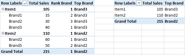
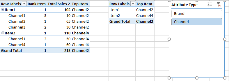
I'm looking for the largest "Brand" and "Channel" within each Item (based on sum of sales). So if I do this manually, I would create two additional pivot tables to summarize by Item-Brand and Item-Channel, like this
<tbody>
</tbody>
<tbody>
</tbody>
I would then create a table with just unique item numbers, and use Index-Match or Vlookup to return the top items in each list.
<tbody>
</tbody>
Clearly, not very efficient and also I frequently need to add/remove columns (i.e. I might be looking for Brand/Channel today but next month need to add something else like customer or market).
I feel as if Power Query could help me here but I am struggling to find an efficient way. The best thought I have so far would be to load the table to PQ, then group by Item-Brand, sort descending by sales, and then remove duplicates. But this is still inefficient because I would need one query for every field I want to find the top item. It would be great to have it all in one query.
Hoping someone might know of a better way.
Thanks
| Item | Brand | Channel | Sales |
| Item1 | Brand1 | Channel1 | 10 |
| Item1 | Brand1 | Channel2 | 25 |
| Item1 | Brand2 | Channel3 | 30 |
| Item1 | Brand3 | Channel2 | 40 |
| Item2 | Brand5 | Channel1 | 50 |
| Item2 | Brand2 | Channel4 | 60 |
<tbody>
</tbody>
I'm looking for the largest "Brand" and "Channel" within each Item (based on sum of sales). So if I do this manually, I would create two additional pivot tables to summarize by Item-Brand and Item-Channel, like this
| Item | Brand | Sum of Sales |
| Item1 | Brand3 | 40 |
| Item1 | Brand1 | 35 |
| Item1 | Brand2 | 30 |
| Item2 | Brand2 | 60 |
| Item2 | Brand5 | 50 |
| Grand Total | 215 |
<tbody>
</tbody>
| Item | Channel | Sum of Sales |
| Item1 | Channel2 | 65 |
| Item1 | Channel3 | 30 |
| Item1 | Channel1 | 10 |
| Item2 | Channel4 | 60 |
| Item2 | Channel1 | 50 |
| Grand Total | 215 |
<tbody>
</tbody>
I would then create a table with just unique item numbers, and use Index-Match or Vlookup to return the top items in each list.
| Item | Top Brand | Top Channel |
| Item1 | Brand3 | Channel2 |
| Item2 | Brand2 | Channel4 |
<tbody>
</tbody>
Clearly, not very efficient and also I frequently need to add/remove columns (i.e. I might be looking for Brand/Channel today but next month need to add something else like customer or market).
I feel as if Power Query could help me here but I am struggling to find an efficient way. The best thought I have so far would be to load the table to PQ, then group by Item-Brand, sort descending by sales, and then remove duplicates. But this is still inefficient because I would need one query for every field I want to find the top item. It would be great to have it all in one query.
Hoping someone might know of a better way.
Thanks
Last edited: