How do I create a Pop-up Notification/Reminder in Excel?

[excelnewbie999]

Hello everyone,

I'm hoping someone can help me with a bit of dilemma. I have a long list of cases that I am working on. I have to be reminded on which ones to chase everyday. I have used conditional formatting where certain cases are coloured which kind of helps, but as the list gets longer, it's difficult to keep up with the coloured cells, , especially when my vision is weak.

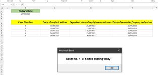
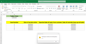
Therefore I feel the best way forward is to have Excel show a notification/reminder that pop-ups based on a date that I have entered. I know this requires a VB script, but not sure how to do this. I'd be very grateful if you could assist me. Please see the below example spreadsheet where cases 1,3,5 show a pop-up in Excel. Any questions, please ask away. Thank you.

Example of Reminder Spreadsheet.xlsx
	B
5	Case Number
Sheet1

 

[Herakles]

I'm once again really sorry Jaafar - I have already tried this, but it's not working. Being a newbie, I'm not sure what to do. Do I need to force Excel to run a macro or something?

View attachment 98149

Have you closed the workbook and opened it again?

 

[Jaafar Tribak]

Have you closed the workbook and opened it again?

Save the workbook and close it. The code should execute automatically when re-opening the workbook.

 

[Jaafar Tribak]

BTW, the code needs a small tweak in order to work when Sheet1 is not the active sheet.

So please, ignore the previous code and use the following update which correctly fully qualifies the ranges.

Option Explicit

Private Sub Workbook_Open()
    'Assumes target sheet is *Sheet1* - change sheet as required.
    Call NotifyUser(Sheet1)
End Sub

Private Sub NotifyUser(ByVal Sh As Worksheet)
    Dim vData() As Variant
    Dim sFiltered() As String
    Dim sNotification As String, sSheetName As String
    Dim lLastRow As Long, lUpperBound As Long, i As Long
    
    sSheetName = Sh.Name
    lLastRow = Sh.Columns("E").Cells(Sh.Rows.Count, 1&).End(xlUp).Row
    vData = Application.Transpose(Evaluate("""|""&" & "INDEX((" & sSheetName & "!E6:E" & lLastRow & ")=" & sSheetName & "!B2,)*ROW(" & sSheetName & "!E6:E" & lLastRow & ")" & "&""|"""))
    sFiltered = Filter(vData, "|0|", False)
    lUpperBound = UBound(sFiltered)
    If lUpperBound <> -1& Then
        For i = 0& To lUpperBound
            sNotification = sNotification & Replace(sFiltered(i), "|", "") - 5& & IIf(i = lUpperBound, "", " - ")
        Next i
        MsgBox "Following case number(s) need chasing today !! " & vbCrLf & vbCrLf & sNotification, vbExclamation
    End If
End Sub

 

[excelnewbie999]

OMG! What an idiot I am! I'm so sorry, but I've now realised what I did wrong.

On the left-side, I simply selected 'ThisWorkbook' and pasted the code. To my realisation now, this was still simply pasting it in 'Sheet1'. As shown below, to resolve the issue, I needed to double-click 'ThisWorkbook' which pops up an actual windows called 'ThisWorkbook (Code)'.

The excel file is now working perfectly, so a very very BIG thank you!

I only have two minor (hopefully) requests if it's possible. How can I:-

1. Change the pop-up so that rather than say for example '2-4', it puts commas after each case number? So for example it's says '2, 4, 5'
2. Simultaneously highlight with colour those cases in the table?

Once again I can't thank you enough!

 

[Jaafar Tribak]

1. Change the pop-up so that rather than say for example '2-4', it puts commas after each case number? So for example it's says '2, 4, 5'

Change this :
For i = 0& To lUpperBound
sNotification = sNotification & Replace(sFiltered(i), "|", "") - 5& & IIf(i = lUpperBound, "", " - ")
Next i

changes in red.
To this :
For i = 0& To lUpperBound
sNotification = sNotification & Replace(sFiltered(i), "|", "") - 5& & IIf(i = lUpperBound, "", " , ")
Next i

2. Simultaneously highlight with colour those cases in the table?

I thought you said you were using Conditional Formatting. The Conditional Formatting should take care of the highlighting of those cases.

BTW, in case you didn't read my last post, please, don't use the first code I posted. Instead, use the last one (in post#13)

 

[excelnewbie999]

That's works absolutely perfect and over the moon - so a big thank you @Jaafar Tribak !!

One thing I would like to know is would the code break if I changed cell names locations etc? If so, how can I make the code more flexible so that if there is a change it can follow through? Or is that not possible?

 

[Jaafar Tribak]

One thing I would like to know is would the code break if I changed cell names locations etc? If so, how can I make the code more flexible so that if there is a change it can follow through? Or is that not possible?

Yes. You can define those cells as module level constants so you can flexibly change them dynamically without needing to modify anything in the NotifyUser routine.

Const SHEET_NAME = "Sheet1!" <== Target sheet name (Don't forget to add the ! char at the end)
Const TODAY_RANGE_ADDRESS = SHEET_NAME & "B2" <== The cell holding the today's date.
Const REMINDER_START_RANGE_ADDRESS = SHEET_NAME & "E6" <== The first cell in the Reminder\Notification popup column.

Option Explicit

'Change these module level Constants as required.
Const SHEET_NAME = "Sheet1!"
Const TODAY_RANGE_ADDRESS = SHEET_NAME & "B2"
Const REMINDER_START_RANGE_ADDRESS = SHEET_NAME & "E6"

Private Sub Workbook_Open()
    Call NotifyUser
End Sub

Private Sub NotifyUser()
    Dim vData() As Variant
    Dim sFiltered() As String
    Dim sNotification As String, sSheetName As String, sReminderAddrs As String
    Dim lLastRow As Long, lUpperBound As Long, i As Long
   
    sSheetName = Replace(SHEET_NAME, "!", "")
    With Sheets(sSheetName)
        lLastRow = .Columns("E").Cells(.Rows.Count, 1&).End(xlUp).Row
    End With
    sReminderAddrs = REMINDER_START_RANGE_ADDRESS & ":E"
    vData = Application.Transpose _
           (Evaluate("""|""&" & "INDEX((" & sReminderAddrs & lLastRow & ")=" & _
           TODAY_RANGE_ADDRESS & ",)*ROW(" & sReminderAddrs & lLastRow & ")" & "&""|"""))
    sFiltered = Filter(vData, "|0|", False)
    lUpperBound = UBound(sFiltered)
    If lUpperBound <> -1& Then
        For i = 0& To lUpperBound
            sNotification = sNotification & Replace(sFiltered(i), "|", "") - 5& & IIf(i = lUpperBound, "", " , ")
        Next i
        MsgBox "Following case number(s) need chasing today !! " & vbCrLf & vbCrLf & sNotification, vbExclamation
    End If
End Sub

 

[excelnewbie999]

Thanks very much. I'm getting a 'Run-time error '9': Subscript out of range. When I press Debug, the following line is highlighted:-

 

[excelnewbie999]

Sorry, the above might be happening because I changed the sheet tab name from Sheet1 to Cases to be worked on

 

[Jaafar Tribak]

Sorry, the above might be happening because I changed the sheet tab name from Sheet1 to Cases to be worked on

That's the purpose of using module level constants.

If you change the name of the sheet, you will need to also change the value of the SHEET_NAME constant to reflect the change .. and the same applies to the other two constants.

Say for example, you changed the Today's date cell from B2 to B3, then you will need to also change:

This:
Const TODAY_RANGE_ADDRESS = SHEET_NAME & "B2"

To this:
Const TODAY_RANGE_ADDRESS = SHEET_NAME & "B3"

You only need to to change the values of the module level constants once and you won't need to change anything in or mess with the NotifyUser routine.