Sumifs using unique and filter functions

[Tarek78]

Hi Everyone,

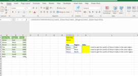
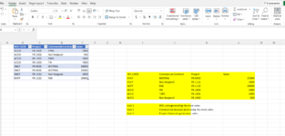
I have attached a spreadsheet and highlighted in yellow the column K I would need to be filled with a formula (spill formula only so that it is completely automated).

Column I and J: This is a spill formula using Unique, Filter and Choose function.
Column K: I would need a spill formula to get the sum of the sales generated by each rep for each region covered


I tried a lot to work on it but cannot find an answer

Thanks for your help

 

[TylerWhieler]

Hi there,

That's a hard one which I don't know if it's even possible.
But I've another solution which can work just fine in automation.

=IF(I6="";"";SUM(UNIQUE(FILTER(C:C;A:A&B:B=I6&J6))))

If you pull the formulla down 4 rows u should be good.
It will always have the same lengt as your spill range.

Hope it helps, GL

 

[Eric W]

Consider:

Book1
	A	B	C	D	E	F	G	H	I	J	K	L	M
1	Sales Rep	Region	Sales						Sales Rep
2	Simon	East	1000						Simon
3	Simon	West	2000
4	Simon	North	1000						Rep	Region	Sales		Sales
5	Tim	South	4000						Simon	East	1000		1000
6	Tim	East	5000						Simon	West	2000		2000
7	Tim	West	1000						Simon	North	1000		1000
8	Nick	South	4000
9	Nick	West	1000
Sheet5

Cell Formulas
Range	Formula
I5:K7	I5	=UNIQUE(FILTER(CHOOSE({1,2,3},Table1_2[Sales Rep],Table1_2[Region],SUMIFS(Table1_2[Sales],Table1_2[Sales Rep],I2,Table1_2[Region],Table1_2[Region])),Table1_2[Sales Rep]=I2))
M5:M7	M5	=SUMIFS(Table1_2[Sales],Table1_2[Sales Rep],INDEX(I5#,0,1),Table1_2[Region],INDEX(I5#,0,2))
Dynamic array formulas.

You can include the sales totals in your original formula if you want (I5), or if you want a separate formula, the M5 formula will work for you.

 

[Tarek78]

Consider:

Book1
	A	B	C	D	E	F	G	H	I	J	K	L	M
1	Sales Rep	Region	Sales						Sales Rep
2	Simon	East	1000						Simon
3	Simon	West	2000
4	Simon	North	1000						Rep	Region	Sales		Sales
5	Tim	South	4000						Simon	East	1000		1000
6	Tim	East	5000						Simon	West	2000		2000
7	Tim	West	1000						Simon	North	1000		1000
8	Nick	South	4000
9	Nick	West	1000
Sheet5

Cell Formulas
Range	Formula
I5:K7	I5	=UNIQUE(FILTER(CHOOSE({1,2,3},Table1_2[Sales Rep],Table1_2[Region],SUMIFS(Table1_2[Sales],Table1_2[Sales Rep],I2,Table1_2[Region],Table1_2[Region])),Table1_2[Sales Rep]=I2))
M5:M7	M5	=SUMIFS(Table1_2[Sales],Table1_2[Sales Rep],INDEX(I5#,0,1),Table1_2[Region],INDEX(I5#,0,2))
Dynamic array formulas.

You can include the sales totals in your original formula if you want (I5), or if you want a separate formula, the M5 formula will work for you.

Thanks for your help . I will try it and let you know if it works. The reason I am creating this is that, ultimately, I want to sort the result by the biggest salesman (Regardless of the region). Would you formula allow me to do that afterwards ?

 

[Eric W]

Sure, a variation of that formula would work:

Book1
	A	B	C	D	E	F
1	Sales Rep	Region	Sales
2	Simon	East	1000
3	Simon	West	2000
4	Simon	North	1000		Rep	Total Sales
5	Tim	South	4000		Tim	10000
6	Tim	East	5000		Nick	5000
7	Tim	West	1000		Simon	4000
8	Nick	South	4000
9	Nick	West	1000
Sheet5

Cell Formulas
Range	Formula
E5:F7	E5	=LET(r,UNIQUE(Table1_2[Sales Rep]),SORT(CHOOSE({1,2},r,SUMIFS(Table1_2[Sales],Table1_2[Sales Rep],r)),2,-1))
Dynamic array formulas.

 

[Tarek78]

Hi there,

That's a hard one which I don't know if it's even possible.
But I've another solution which can work just fine in automation.

=IF(I6="";"";SUM(UNIQUE(FILTER(C:C;A:A&B:B=I6&J6))))

If you pull the formulla down 4 rows u should be good.
It will always have the same lengt as your spill range.

Hope it helps, GL
View attachment 66243
View attachment 66244

Thanks I will try it and let you know

 

[Tarek78]

Hi Everyone,

First of all, I would like to thank you all for helping. It is much appreciated.
I couldn't find an answer to my reply but I think my description wasn't clear enough so I will try explain it better this time.

I have attached a picture as I don't know how to install the XL2BB add-in.


We have the raw data in the table (column B to E).

I want a dynamic array formula (unique, filter, choose etc.) that gives me 4 columns :

- Column 1= IRIS CODE which is the account
- Column 2= Commercial contract which can be a sum of various project code
- Column 3= Project Code
- Column 4= Sales generated


I want the formula to sort this result ideally in this order (as specified in the yellow section):

1- the account generating the most sales
2- the commercial contract generating the most sales
3- the project generating the most sales


I don't if it is possible to perfom 3 sorts but if it is not, let me know


Thanks again so much for your help

 

[Tarek78]

Hi Everyone,

I was wondering if someone found a solution?

 

[Alex Blakenburg]

Any reason you don't just use a pivot table ?

20220605 Filter Unique Sort or Pivot Tarek78.xlsx
	A	B	C	D	E	F	G	H	I	J
1	IRIS CODE	Project	Commercial Contract	Sales			IRIS CODE	Commercial Contract	Project	Sales
2	ACCO	FR.1001	TARS	1000			SNCF	MISTRAL	FR.0400	25000
3	ACCO	FR.1002	Not Assigned	500			SNCF	Not Assigned	FR.1111	3000
4	ACCO	FR.1001	TARS	2000			RATP	RAE	FR.1122	20000
5	ACCO	FR.1003	FRI	4000			ACCO	FRI	FR.1003	4000
6	SNCF	FR.0400	MISTRAL	10000			ACCO	TARS	FR.1001	3000
7	SNCF	FR.0400	MISTRAL	15000			ACCO	Not Assigned	FR.1002	500
8	SNCF	FR.1111	Not Assigned	3000
9	RATP	FR.1122	RAE	20000
Data

 

[Tarek78]

Yes, because I want to format it the way I want with additional info not from the initial raw data