3 level dependant dropdown help (no macros)

[Akira181]

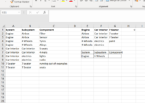
I’m trying to create a dependant dropdown list 3 levels deep. I’ve been trying to avoid all macros to keep it simple but I cannot get the 3rd level to work properly. I tried using offsets to create dynamic named lists, then a combination of the Indirect and Substitute functions in the data validation to create the drop down

One of the problems I'm having is that the named ranges are similar in name and some of them start with a number, making the substitute function not work properly. Can someone tell me the best way to do this without using a macro?

 

[bobsan42]

Start by separaing the validation lists in three tables with the dependecy to the previous level.
This is to avoid duplicates in the first two levels.
I will try to elaborate and suggest a solution later.

 

[Toadstool]

Hi Akira181,

I'm struggling understanding the purpose of E1 to G6 so I'll assume it's just a work area to build the Data Validation lists.
You don't say what version of Excel you use as this would be easier with the latest versions but here's my Excel 2016 approach.

Akira181.xlsx
	A	B	C	D	E	F	G
1	System	Subsystem	Component		System	Subsystem	Component
2	Engine	Airbox	Filter		Engine	Airbox	Tyres
3	Engine	Airbox	Sensor		Car Interior	4 Wheels	Alloys
4	Engine	4 Wheels	Tyres		7 Seater
5	Engine	4 Wheels	Alloys
6	Car Interior	Car Interior	5 Seats
7	Car Interior	Car Interior	4 Mats		System	Subsystem	Component
8	Car Interior	electrics	Lights		Engine	4 Wheels	Alloys
9	Car Interior	electrics	Radio
10	7 Seater	7 Seater	running out of examples
11	7 Seater	7 Seater	seats
12
Example

Cell Formulas
Range	Formula
E2:E6	E2	=IFERROR(INDEX(A$2:A$12,AGGREGATE(15,6,ROW($A$2:$A$12)-ROW($A$1)/((ISNA(MATCH(A$2:A$12,E$1:E1,0)))),1))&"","")
F2:F6	F2	=IFERROR(INDEX(B$2:B$12,AGGREGATE(15,6,ROW($A$2:$A$12)-ROW($A$1)/((ISNA(MATCH(B$2:B$12,F$1:F1,0))*($A$2:$A$12=$E$8))),1))&"","")
G2:G6	G2	=IFERROR(INDEX(C$2:C$12,AGGREGATE(15,6,ROW($A$2:$A$12)-ROW($A$1)/((ISNA(MATCH(C$2:C$12,G$1:G1,0))*($A$2:$A$12=$E$8)*(B$2:B$12=$F$8))),1))&"","")

Cells with Data Validation
Cell	Allow	Criteria
E8:G8	List	=OFFSET(E$2,,,COUNTIF(E$2:E$6,"> "))

 

[Akira181]

Hi Akira181,

I'm struggling understanding the purpose of E1 to G6 so I'll assume it's just a work area to build the Data Validation lists.
You don't say what version of Excel you use as this would be easier with the latest versions but here's my Excel 2016 approach.

Akira181.xlsx
	A	B	C	D	E	F	G
1	System	Subsystem	Component		System	Subsystem	Component
2	Engine	Airbox	Filter		Engine	Airbox	Tyres
3	Engine	Airbox	Sensor		Car Interior	4 Wheels	Alloys
4	Engine	4 Wheels	Tyres		7 Seater
5	Engine	4 Wheels	Alloys
6	Car Interior	Car Interior	5 Seats
7	Car Interior	Car Interior	4 Mats		System	Subsystem	Component
8	Car Interior	electrics	Lights		Engine	4 Wheels	Alloys
9	Car Interior	electrics	Radio
10	7 Seater	7 Seater	running out of examples
11	7 Seater	7 Seater	seats
12
Example

Cell Formulas
Range	Formula
E2:E6	E2	=IFERROR(INDEX(A$2:A$12,AGGREGATE(15,6,ROW($A$2:$A$12)-ROW($A$1)/((ISNA(MATCH(A$2:A$12,E$1:E1,0)))),1))&"","")
F2:F6	F2	=IFERROR(INDEX(B$2:B$12,AGGREGATE(15,6,ROW($A$2:$A$12)-ROW($A$1)/((ISNA(MATCH(B$2:B$12,F$1:F1,0))*($A$2:$A$12=$E$8))),1))&"","")
G2:G6	G2	=IFERROR(INDEX(C$2:C$12,AGGREGATE(15,6,ROW($A$2:$A$12)-ROW($A$1)/((ISNA(MATCH(C$2:C$12,G$1:G1,0))*($A$2:$A$12=$E$8)*(B$2:B$12=$F$8))),1))&"","")

Cells with Data Validation
Cell	Allow	Criteria
E8:G8	List	=OFFSET(E$2,,,COUNTIF(E$2:E$6,"> "))

Yeah, it was just a working area to try and build the lists, should have mentioned. Also, I'm using Office 365. I figured it out in the end using Indirect(substitiute(xx)) for the second level and the solution here (also your post!) for the third level how to create dependent dropdown list in Excel

I feel like it could be done cleaner but I've spent too much time messing around to continue trying. It works so that's good enough for me. Thanks!

 

[Toadstool]

You're welcome.

 

[Akira181]

You're welcome.

Actually, I've noticed a slight problem

The dropdown lists starting in E8 will have multiple lines but the formula you posted works for one row. Can it be modified?

 

[Toadstool]

The question was presented with one row for dropdowns. If you want more then the System can be created in one place but the data list for the Subsystem and Component dropdowns will need to be built for each row.

What is the maximum number of unique entries for Subsystem and Component?
How many rows of dropdowns are needed?
I can then use the columns to the right of G to build the selection lists... but the execution time will increase with large numbers.

 

[Akira181]

The question was presented with one row for dropdowns. If you want more then the System can be created in one place but the data list for the Subsystem and Component dropdowns will need to be built for each row.

What is the maximum number of unique entries for Subsystem and Component?
How many rows of dropdowns are needed?
I can then use the columns to the right of G to build the selection lists... but the execution time will increase with large numbers.

I managed to build the data lists by modifying the formula you posted in the other thread. I was just wondering if there was a way to do it without building the lists but no matter, it works so not going to spend anymore time on it.

Thanks!

 

[Toadstool]

You're welcome.
Glad you got it to work. I don't think there's a more elegant way unless you're using 365 or resort to VBA.