Accounting trial balance

[gsm2000]

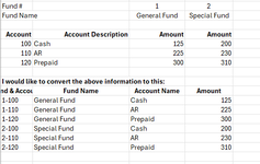
I have an accounting trial balance that I would like to convert from showing the funds in columns and accounts in rows, to the information being combined (I've shown only 2 columns/funds for simplicity but in reality there would be over 100 funds and over 100 accounts). Thanks in advance!

 

[KRice]

Are you familiar with Power Query? You can transform the upper data set using various operations. I would recommend operating on a copy of your original worksheet, and leave the original untouched. Power Query (PQ) will take data from a table or range and load it into a separate application built into Excel. But the first step will automatically convert a range of data into an official Excel table. I'm assuming your actual data set mimics the structure presented...two header rows followed by a blank row followed by another header row followed by the actual data. And for the columns...everything in the same order shown here...

MrExcel_20240305.xlsx
	A	B	C	D
4	Fund #		1	2
5	Fund Name		General Fund	Special Fund
6
7	Account	Account Description	Amount	Amount
8	100	Cash	125	200
9	110	AR	225	230
10	120	Prepaid	300	310
gsm2000

Click on a cell somewhere inside the upper table range and then Data > Get & Transform Data submenu > From Table/Range (a small table icon). You should see a popup window with a suggestion for the entire range to take...confirm the range is correct and indicate that you do not have headers (do not check the box). The range will be converted to a table with headers of Column1, Column2, etc. And PQ will launch and your table will be imported into it. You should have columns 1 and 2 showing Account and Account Description followed by Columns 3...with the various funds. This establishes the connection between your Excel table and Power Query. Now for the shortcut...open the advanced editor in PQ (View > Advanced Editor) and you'll see the M Code...looking something like this. Note the name of the Table where you see Name="Table5" here...yours might have a different table name. Note that name, then delete all of your M Code and replace it with the code further below...and edit the first Source line to reflect the same table name that you had originally.

let
    Source = Excel.CurrentWorkbook(){[Name="Table5"]}[Content],
    #"Changed Type" = Table.TransformColumnTypes(Source,{{"Column1", type any}, {"Column2", type text}, {"Column3", type any}, {"Column4", type any}})
in
    #"Changed Type"

Change the Name="Table... " name to yours...

let
    Source = Excel.CurrentWorkbook(){[Name="Table1"]}[Content],
    #"Changed Type" = Table.TransformColumnTypes(Source,{{"Column1", type text}}),
    #"Added Custom1" = Table.AddColumn(#"Changed Type", "Custom", each [Column1]&"|"&[Column2]),
    #"Removed Columns2" = Table.RemoveColumns(#"Added Custom1",{"Column1", "Column2"}),
    #"Transposed Table" = Table.Transpose(#"Removed Columns2"),
    #"Changed Type2" = Table.TransformColumnTypes(#"Transposed Table",{{"Column1", type text}}),
    #"Added Custom2" = Table.AddColumn(#"Changed Type2", "Custom", each [Column1]&"|"&[Column2]),
    #"Removed Columns" = Table.RemoveColumns(#"Added Custom2",{"Column3", "Column1", "Column2"}),
    #"Renamed Columns1" = Table.RenameColumns(#"Removed Columns",{{"Custom", "Column1"}}),
    #"Reordered Columns" = Table.ReorderColumns(#"Renamed Columns1", List.Sort( Table.ColumnNames(#"Renamed Columns1"), Order.Ascending )),
    #"Transposed Table1" = Table.Transpose(#"Reordered Columns"),
    #"Promoted Headers" = Table.PromoteHeaders(#"Transposed Table1", [PromoteAllScalars=true]),
    #"Unpivoted Other Columns" = Table.UnpivotOtherColumns(#"Promoted Headers", {"Column3"}, "Attribute", "Value"),
    #"Split Column by Delimiter" = Table.SplitColumn(#"Unpivoted Other Columns", "Column3", Splitter.SplitTextByDelimiter("|", QuoteStyle.Csv), {"Column3.1", "Column3.2"}),
    #"Changed Type1" = Table.TransformColumnTypes(#"Split Column by Delimiter",{{"Column3.1", type text}, {"Column3.2", type text}}),
    #"Split Column by Delimiter1" = Table.SplitColumn(#"Changed Type1", "Attribute", Splitter.SplitTextByDelimiter("|", QuoteStyle.Csv), {"Attribute.1", "Attribute.2"}),
    #"Added Custom" = Table.AddColumn(#"Split Column by Delimiter1", "Custom", each [Attribute.1]&"-"&[Column3.1]),
    #"Removed Columns1" = Table.RemoveColumns(#"Added Custom",{"Column3.1", "Attribute.1"}),
    #"Reordered Columns1" = Table.ReorderColumns(#"Removed Columns1",{"Custom", "Column3.2", "Attribute.2", "Value"}),
    #"Renamed Columns" = Table.RenameColumns(#"Reordered Columns1",{{"Custom", "Fund & Account"}, {"Column3.2", "Account Name"}, {"Attribute.2", "Fund Name"}, {"Value", "Amount"}}),
    #"Removed Top Rows" = Table.Skip(#"Renamed Columns",2),
    #"Sorted Rows" = Table.Sort(#"Removed Top Rows",{{"Fund & Account", Order.Ascending}}),
    #"Reordered Columns2" = Table.ReorderColumns(#"Sorted Rows",{"Fund & Account", "Fund Name", "Account Name", "Amount"})
in
    #"Reordered Columns2"

After editing the M code, confirm it with Done. You can then step through the various steps if desired using the Applied Steps pane to the right. By the time you reach the last step, you should have the desired final form. To load this back into Excel, choose File > Close & Load...and you'll probably want to specify that you want a Table delivered to a New Worksheet...and then you should be taken back into Excel where you'll see something like this:

MrExcel_20240305.xlsx
	A	B	C	D
1	Fund & Account	Fund Name	Account Name	Amount
2	1-100	General Fund	Cash	125
3	1-110	General Fund	AR	225
4	1-120	General Fund	Prepaid	300
5	2-100	Special Fund	Cash	200
6	2-110	Special Fund	AR	230
7	2-120	Special Fund	Prepaid	310
gsm2000_output

To refresh this, anytime the source table is updated, go to the output table, select any cell in it and click Data > Refresh ...or Data > Refresh All from anywhere in the workbook.

You can do this with some complex formulas in Excel, but Power Query might be easier in this case.

 

[Ezguy4u]

Krice because you can never have too many solutions, here is another one.

Sub Prog1()

Dim CntCol As Long
Dim CntAcct As Long
Dim Row1 As Long

CntAcct = 1
Row1 = 13
Row2 = 13

CntCol = Cells(6, Columns.Count).End(xlToLeft).Column

For i = 1 To CntCol

Cells(6, i).Select

Cells(Row1, 1) = CntAcct & "-" & 100
Cells(Row1 + 1, 1) = CntAcct & "-" & 110
Cells(Row1 + 2, 1) = CntAcct & "-" & 120

Cells(Row1, 2) = Cells(4, i + 2)
Cells(Row1 + 1, 2) = Cells(4, i + 2)
Cells(Row1 + 2, 2) = Cells(4, i + 2)

Cells(Row1, 3) = Cells(7, 2)
Cells(Row1 + 1, 3) = Cells(8, 2)
Cells(Row1 + 2, 3) = Cells(9, 2)

Cells(Row1, 4) = Cells(7, i + 2)
Cells(Row1 + 1, 4) = Cells(8, i + 2)
Cells(Row1 + 2, 4) = Cells(9, i + 2)

CntAcct = CntAcct + 1
Row1 = Row1 + 3

Next i

End Sub

24-03-07 1.xlsm
	A	B	C	D
1
2
3	Fund #		1	2
4	Fund Name		General Fund	Special Fund
5
6	Account	Account Description	Amount	Amount
7	100	Cash	125	200
8	110	AR	225	230
9	120	Prepaid	300	310
10
11
12	Fund & Account	Fund Name	Account Name	Amount
13	1-100	General Fund	Cash	125
14	1-110	General Fund	AR	225
15	1-120	General Fund	Prepaid	300
16	2-100	Special Fund	Cash	200
17	2-110	Special Fund	AR	230
18	2-120	Special Fund	Prepaid	310
Data

 

[Peter_SSs]

You can do this with some complex formulas in Excel, but Power Query might be easier in this case.

To me, this formula approach is much simpler than that Power Query code and instructions.

@gsm2000
Welcome to the MrExcel board!
If you are interested in a formula approach you just need these 4 formulas across the top row of the results.

24 03 08.xlsm
	A	B	C	D
1
2
3	Fund #		1	2
4	Fund Name		General Fund	Special Fund
5
6	Account	Account Description	Amount	Amount
7	100	Cash	125	200
8	110	AR	225	230
9	120	Prepaid	300	310
10
11
12	Fund & Account	Fund Name	Account Name	Amount
13	1-100	General Fund	Cash	125
14	1-110	General Fund	AR	225
15	1-120	General Fund	Prepaid	300
16	2-100	Special Fund	Cash	200
17	2-110	Special Fund	AR	230
18	2-120	Special Fund	Prepaid	310
gsm2000

Cell Formulas
Range	Formula
A13:A18	A13	=TOCOL(C3:D3&"-"&A7:A9,,1)
B13:B18	B13	=XLOOKUP(--TEXTBEFORE(A13#,"-"),C3:D3,C4:D4)
C13:C18	C13	=XLOOKUP(--TEXTAFTER(A13#,"-"),A7:A9,B7:B9)
D13:D18	D13	=TOCOL(C7:D9,,1)
Dynamic array formulas.

For your much larger ranges you just need to increase the ranges in the 4 formulas. For example I did a test with 119 funds from col C to col DQ and 104 accounts from row 7 to row 110 and these are the expanded formulas.

24 03 08.xlsm
	A	B	C	D
113	Fund & Account	Fund Name	Account Name	Amount
114	1-100	General Fund	Cash	421
gsm2000 (2)

Cell Formulas
Range	Formula
A114:A12489	A114	=TOCOL(C3:DQ3&"-"&A7:A110,,1)
B114:B12489	B114	=XLOOKUP(--TEXTBEFORE(A114#,"-"),C3:DQ3,C4:DQ4)
C114:C12489	C114	=XLOOKUP(--TEXTAFTER(A114#,"-"),A7:A110,B7:B110)
D114:D12489	D114	=TOCOL(C7:DQ110,,1)
Dynamic array formulas.

 

[KRice]

Oh, my morning entertainment...see better options than my messy PQ solution, @Ezguy4u and @Peter_SSs, thank you both for weighing in with great options!

 

[gsm2000]

Thank you all! I appreciate your time and your responses on this. This is extremely helpful.

 

[gsm2000]

To me, this formula approach is much simpler than that Power Query code and instructions.

@gsm2000
Welcome to the MrExcel board!
If you are interested in a formula approach you just need these 4 formulas across the top row of the results.

24 03 08.xlsm
	A	B	C	D
1
2
3	Fund #		1	2
4	Fund Name		General Fund	Special Fund
5
6	Account	Account Description	Amount	Amount
7	100	Cash	125	200
8	110	AR	225	230
9	120	Prepaid	300	310
10
11
12	Fund & Account	Fund Name	Account Name	Amount
13	1-100	General Fund	Cash	125
14	1-110	General Fund	AR	225
15	1-120	General Fund	Prepaid	300
16	2-100	Special Fund	Cash	200
17	2-110	Special Fund	AR	230
18	2-120	Special Fund	Prepaid	310
gsm2000

Cell Formulas
Range	Formula
A13:A18	A13	=TOCOL(C3:D3&"-"&A7:A9,,1)
B13:B18	B13	=XLOOKUP(--TEXTBEFORE(A13#,"-"),C3:D3,C4:D4)
C13:C18	C13	=XLOOKUP(--TEXTAFTER(A13#,"-"),A7:A9,B7:B9)
D13:D18	D13	=TOCOL(C7:D9,,1)
Dynamic array formulas.

For your much larger ranges you just need to increase the ranges in the 4 formulas. For example I did a test with 119 funds from col C to col DQ and 104 accounts from row 7 to row 110 and these are the expanded formulas.

24 03 08.xlsm
	A	B	C	D
113	Fund & Account	Fund Name	Account Name	Amount
114	1-100	General Fund	Cash	421
gsm2000 (2)

Cell Formulas
Range	Formula
A114:A12489	A114	=TOCOL(C3:DQ3&"-"&A7:A110,,1)
B114:B12489	B114	=XLOOKUP(--TEXTBEFORE(A114#,"-"),C3:DQ3,C4:DQ4)
C114:C12489	C114	=XLOOKUP(--TEXTAFTER(A114#,"-"),A7:A110,B7:B110)
D114:D12489	D114	=TOCOL(C7:DQ110,,1)
Dynamic array formulas.

Peter_SSs
This formula works perfectly - this is such a timesaver for a couple of projects that I do!
Would you mind clarifying one thing - I've tried to look this up and still am not exactly sure what exactly is the purpose of the "--" prior to the textbefore? I can see that the formula won't work without it, but just curious as to exactly what it is doing. Thanks so much for your help.

 

[KRice]

The double unary operator (--) is being used in this case to operate on the text that spills down the A column. TEXTBEFORE and TEXTAFTER are isolating the value before and after the hyphen in the Fund & Account list, but the values are still considered to be text, not numbers. Peter's clever formula wants these text values converted back into numbers so that they can be used to matchup with the Fund # and Account numbers, both consist of numeric values, not text. To do that the double unary is used, which effectively multiplies the text (that appears to be a number but is still text) by -1, and the multiplication coerces Excel into treating the text as a number, although it is now a negative number. So a second multiplication by -1 is done,,. the other "-", which now gives the correct sign. You could achieve the same result with 1* instead of --, as the first multiplication is what coerces the text to numbers.

 

[gsm2000]

The double unary operator (--) is being used in this case to operate on the text that spills down the A column. TEXTBEFORE and TEXTAFTER are isolating the value before and after the hyphen in the Fund & Account list, but the values are still considered to be text, not numbers. Peter's clever formula wants these text values converted back into numbers so that they can be used to matchup with the Fund # and Account numbers, both consist of numeric values, not text. To do that the double unary is used, which effectively multiplies the text (that appears to be a number but is still text) by -1, and the multiplication coerces Excel into treating the text as a number, although it is now a negative number. So a second multiplication by -1 is done,,. the other "-", which now gives the correct sign. You could achieve the same result with 1* instead of --, as the first multiplication is what coerces the text to numbers.

Awesome, that is really helpful. Thanks for the clarification!

 

[Peter_SSs]

Peter_SSs
This formula works perfectly - this is such a timesaver for a couple of projects that I do!

You are welcome. Thanks for the follow-up.

.. and just to add a little to Kirk's explanation about converting the TEXTBEFORE and TEXTAFTER values to numerical values to match the numerical values in row 3 and column A:
We could just as easily gone the other way and left the TEXTBEFORE and TEXTAFTER values as text and instead converted the row 3 and column A numerical values to text so they matched that way.
So removing the red and adding the blue would do that
=XLOOKUP(--TEXTBEFORE(A13#,"-"),C3:D3,C4:D4)
=XLOOKUP(TEXTBEFORE(A13#,"-"),C3:D3&"",C4:D4)

Here it is in action in the col B & C formulas.

24 03 08.xlsm
	A	B	C	D
3	Fund #		1	2
4	Fund Name		General Fund	Special Fund
5
6	Account	Account Description	Amount	Amount
7	100	Cash	125	200
8	110	AR	225	230
9	120	Prepaid	300	310
10
11
12	Fund & Account	Fund Name	Account Name	Amount
13	1-100	General Fund	Cash	125
14	1-110	General Fund	AR	225
15	1-120	General Fund	Prepaid	300
16	2-100	Special Fund	Cash	200
17	2-110	Special Fund	AR	230
18	2-120	Special Fund	Prepaid	310
gsm2000 (3)

Cell Formulas
Range	Formula
A13:A18	A13	=TOCOL(C3:D3&"-"&A7:A9,,1)
B13:B18	B13	=XLOOKUP(TEXTBEFORE(A13#,"-"),C3:D3&"",C4:D4)
C13:C18	C13	=XLOOKUP(TEXTAFTER(A13#,"-"),A7:A9&"",B7:B9)
D13:D18	D13	=TOCOL(C7:D9,,1)
Dynamic array formulas.