active cell

[charly1]

hi all

I am relatively new to excel, so my question may indeed be a simple one.

I would like to write a "xlookup formula" in which the "lookup value" is constantly updated to refer to the "activecell". Is this possible without using vba and without having to double click the active cell to update the reference in the cell containing the xlookup formula?

Any help would be greatly appreciated!

 

[Fluff]

No it's not possible without VBA.

 

[charly1]

Ok.

So would it be to much to ask for someone out there to post the necessary vba code that I need.

I would like to insert the xlookup code into cell "A1" of sheet1, the lookup value would always be the active cell. The lookup array should refer to a Table column on that same sheet 1 and the return array should be 2 side by side columns in a separate table in sheet 2.

Thanks ever so much for any help in advance.

 

[charly1]

sorry, if may just add one final point to my q. I would like the vba to only run the xlookup when the active cell happens to be a cell in a specific column of an excel table.

 

[Joe4]

It is hard to tailor VBA to work on your specific situation without detailed information.
Please show us some sample data and your expected results.

MrExcel has a tool called “XL2BB” that lets you post samples of your data that will allow us to copy/paste it to our Excel spreadsheets, so we can work with the same copy of data that you are. Instructions on using this tool can be found here: XL2BB Add-in

Note that there is also a "Test Here” forum on this board. This is a place where you can test using this tool (or any other posting techniques that you want to test) before trying to use those tools in your actual posts.

 

[charly1]

It is hard to tailor VBA to work on your specific situation without detailed information.
Please show us some sample data and your expected results.

MrExcel has a tool called “XL2BB” that lets you post samples of your data that will allow us to copy/paste it to our Excel spreadsheets, so we can work with the same copy of data that you are. Instructions on using this tool can be found here: XL2BB Add-in

Note that there is also a "Test Here” forum on this board. This is a place where you can test using this tool (or any other posting techniques that you want to test) before trying to use those tools in your actual posts.

Hi

thanks for answering.

I have copied the sample data below. The xlookup appears in cell A1. I would like to have that formula for that cell written in vba, where lookup value is not cell P190 as it currently stands but to rather to always refer to the active cell - provided the active cell is in the table column P. All other data in the above function is to remain the same.

Please note though, the lookup array and return array refer to columns of a table that appear in a separate spreadsheet of the same workbook.

Thanks again in advance. Any help would be appreciated immensely.

NewCat.xlsm
	A	B	C	D	E	F	G	H	I	J	K	L	M	N	O	P
1	אחרונים	1870	ה' תרל	1921	ה' תרפא	51									ראשונים	1050
2
3	עמודה1	עמוד	מדף	1	Column1	Column2	ספר	חלקים	נושא כללי: בנושאים	נושא פרטי: בנושאים	נושא: בספרים	נושא כללי: בנושאים [שני]	נושא פרטי: בנושאים [שני]	נושא: בספרים [שני]	תוכן	מחבר
4		-	-	ספר ראומה	ד	3	הלכות שחיטות ובדיקות לקדמוני איטליא	0	הלכה	יו"ד: א'-קכ"ב [מאכלות אסורות], פסקי ראשונים וגדולי האחרונים	יו"ד	-	-	-	-	-
5		ח,ט	7	-			טור - מהד' המאור	23	הלכה	ספרי טושו"ע	ספרי טושו"ע	-	-	-	-	-
6		ח	4	-			טור - מהד' שירת דבורה [בינוני]	23	הלכה	ספרי טושו"ע	ספרי טושו"ע	-	-	-	-	-
7		מועדים	מועדים	-			טור - מהד' שירת דבורה [גדול]	21	הלכה	ספרי טושו"ע	ספרי טושו"ע	-	-	-	-	-
8		ח, ט	2	-			טור - מהד' שירת דבורה [קטן]	23	הלכה	ספרי טושו"ע	ספרי טושו"ע	-	-	-	-	-
9		ח, ט	3	-			טור ושו"ע - שירת דבורה [קטן]	38	הלכה	ספרי טושו"ע	ספרי טושו"ע	-	-	-	-	-
10		כט	8	-			מאורות הראשונים	1	הלכה	פסקי ראשונים וגדולי האחרונים	פסקי הראשונים וגדולי האחרונים	-	-	-	-	-
11		-	-	שבלי הלקט - מהדו"י	ד	3	מנהג טוב	0	הלכה	פסקי ראשונים וגדולי האחרונים	פסקי הראשונים וגדולי האחרונים	-	-	-	-	-
12		-	-	משנה ברורה - מהד' דרשו	י	2,3	ספר המפתח [למ"ב] - דרשו	0	הלכה	אורח חיים	אורח חיים	-	-	-	-	-
13		כט	8	-			ספר קושיות	1	הלכה	פסקי ראשונים וגדולי האחרונים	פסקי הראשונים וגדולי האחרונים	-	-	-	-	-
14		ט,י	7	-			שולחן ערוך - מהד' פרידדמן	34	הלכה	ספרי טושו"ע	ספרי טושו"ע	-	-	-	-	-
15		ט	5	-			שולחן ערוך - מהדו"י	10	הלכה	ספרי טושו"ע	ספרי טושו"ע	-	-	-	-	-
16		ח	5	-			שולחן ערוך - צורת הדף	10	הלכה	ספרי טושו"ע	ספרי טושו"ע	-	-	-	-	-
מפתח

Cell Formulas
Range	Formula
A1:F1	A1	=XLOOKUP(P190,ArtistName,Table2[[עמודה2]:[עמודה7]])
O1:P1	O1	=XLOOKUP(P2756,ArtistName,Table2[[עמודה2]:[DOB CAL]])
E4:E16	E4	=IF([@1]="-","",XLOOKUP([@1],[ספר],[עמוד]))
F4:F16	F4	=IF([@1]="-","",XLOOKUP([@1],[ספר],[מדף]))
Dynamic array formulas.

Named Ranges
Name	Refers To	Cells
ArtistName	=מחברים!$A$7:$A$1872	A1:F1, O1:P1
ר__אחא__אחאי__משבחא	=מחברים!$A$8:$A$1872	A1:F1, O1:P1

Cells with Data Validation
Cell	Allow	Criteria
P4:P16	List	=ArtistName

 

[Joe4]

Go to sheet where you want to apply this to (the sheet where you want to update the formula in cell A1), then right-click on the sheet tab name at the bottom of the screen, select "View Code", and paste this VBA code in the VB Editor window that pops-up:

Private Sub Worksheet_SelectionChange(ByVal Target As Range)

'   Check to see if selected cell is in column P under row 3
    If Target.Column = 16 And Target.Row > 3 Then
'       Update formula in cell A1 with address of selected cell
        Range("A1").Formula "=XLOOKUP(" & Target.Address & ",ArtistName,Table2[[עמודה2]:[עמודה7]])"
    End If
    
End Sub

Now, as you pick any cell value in column P beneath row 3, it will populate your lookup formula in cell A1 with the address of that cell.

 

[charly1]

Go to sheet where you want to apply this to (the sheet where you want to update the formula in cell A1), then right-click on the sheet tab name at the bottom of the screen, select "View Code", and paste this VBA code in the VB Editor window that pops-up:

Private Sub Worksheet_SelectionChange(ByVal Target As Range)

'   Check to see if selected cell is in column P under row 3
    If Target.Column = 16 And Target.Row > 3 Then
'       Update formula in cell A1 with address of selected cell
        Range("A1").Formula "=XLOOKUP(" & Target.Address & ",ArtistName,Table2[[עמודה2]:[עמודה7]])"
    End If
   
End Sub

Now, as you pick any cell value in column P beneath row 3, it will populate your lookup formula in cell A1 with the address of that cell.

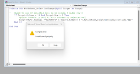
Thanks so much for your time, however it didn't work. I've attached a screenshot showing what happened when I entered it.

 

[charly1]

By the way, for some reason it didn't show up on the screenshot picture attached above, however the word ".formula" in your code washighlighted in blue, when the error message popped up.

Thanks again, for the effort.

 

[Joe4]

Sorry, there is a typo in that code. When I was trying to copy the special characters of your alphabet, I lost an equal sign. It should be:

Private Sub Worksheet_SelectionChange(ByVal Target As Range)

'   Check to see if selected cell is in column P under row 3
    If Target.Column = 16 And Target.Row > 3 Then
'       Update formula in cell A1 with address of selected cell
        Range("A1").Formula = "=XLOOKUP(" & Target.Address & ",ArtistName,Table2[[עמודה2]:[עמודה7]])"
    End If
    
End Sub