Any clever solutions to speed up a 50,000 row MATCH formula?

[d0rian]

I have a data set of 50,000 text entries in column A. Every day a few hundred entries are added to the data set, and I paste the NEW set of entries (e.g. let's say a total of 50,275, which includes both the 50,000 from the prior day and 275 new ones) in column B.
I want the fastest way to identify the new 275 entries (which exist in column B, but not A).
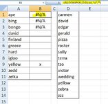
The simplest method I know of is to paste a simple MATCH formula in column C, e.g. =IF(ISNUMBER(MATCH(B1,A:A,0)),"","n")
But that takes 10-12 seconds to run on 50,000+ rows.

Can anyone think of any way to accomplish this faster?

 

[jasonb75]

but that's of course the super-slow formula in the OP I started out with that I presume uses linear logic,

With MATCH (and v / hlookup) the last argument dictates the logic. Using 0 or FALSE means a linear / exact match. Using 1 / TRUE means a binary / approximate match.

In addition to the 2 options that I mention above, MATCH also has an argument of -1 which performs a binary search in reverse order when the data is sorted descending.

X lookup / match in office 365 have slightly different arguments and more flexibility. A couple of things that I have tried didn't work as expected, although that would more likely have been me not using it correctly than a problem with the function.

 

[Alex Blakenburg]

Especially since @jasonb75 mentioned XLookup, you might find the article in the link below interesting.
It mostly compares the performance of Xlookup to Vlookup both Linear and Binary, with a bit of Index/Match thrown in for good measure.
It indicates that XLookup is quite a bit slower in a Linear search but only marginally slower in a Binary search with binary being significantly faster, for both functions.
Performance of XLOOKUP: How fast is the new XLOOKUP vs. VLOOKUP?

 

[GraH]

Found this exact same article yesterday too and wanted to share it today. You just beat me @Alex Blakenburg.

 

[Alex Blakenburg]

@GraH LOL. Like minds. I had it tucked away in my OneNote.

 

[d0rian]

I'm playing around with this syntax and it's been a godsend so far, but I can't understand what's going on in the screenshot below. The highlighted formula is in B1 and copied down through B11.
Why does it return #N/A errors for the first 3 entries? I suppose it "works" in that it correctly identifies "yellow" as the only word that appears in the list in column D, but I don't understand why some of the cells in col B return errors? Col D is sorted alphabetically, which I thought was the only pre-requisite....?

EDIT: yes, I know that #N/A errors are typically returned when a value can't be found in a lookup range, but then why aren't there #N/A errors in col B next to ALL un-found words?

 

[Alex Blakenburg]

I recall Fluff addressing this in another post.
Push your list in column D down 1 row and make the first item in Column D as just "a" (without the quotes)

 

[d0rian]

I recall Fluff addressing this in another post.
Push your list in column D down 1 row and make the first item in Column D as just "a" (without the quotes)

Well that works (thanks) but....why? I have some pretty gnarly data sets I want to use this binary methodology on, but need to understand its quirks before feeling comfortable deploying.

(I also realize that my screenshot has a small mistake in it..."david" is in both columns, but the formula in column B didn't place an "x" next to it...I might have accidentally included an extra trailing space or inadvertently deleted the formula in that row...ignore that inconsistency, though)

EDIT: I tried various strings in cell D1..."a" worked (to get rid of the N/A errors...so did ab, ac, etc etc...all the way up to "ap". "aq", however, produced the NA error...that's significant because you'll notice aq is the first text string that would come AFTER the first word in column A (ape). So the answer has something to do with that...but why should it matter whether the first entry in the lookup range is BEFORE or AFTER the first entry to be searched? I thought that all that mattered is that the lookup range be sorted alphabetically, but there's clearly something slightly more complex going on...?

 

[jasonb75]

but why should it matter whether the first entry in the lookup range is BEFORE or AFTER the first entry to be searched?

Excel comes with a built in help file that tells you this. You can find this help by typing =LOOKUP into excel then pressing the f1 key (don't press enter first). This works with any formula function.

This is an extract from the help page for the LOOKUP function that tells you the reasons for the error that you're seeing and why it works in the way that it does. There is more to read there but this part is most relevant.

Support page

• If the LOOKUP function can't find the lookup_value, the function matches the largest value in lookup_vector that is less than or equal to lookup_value.
• If lookup_value is smaller than the smallest value in lookup_vector, LOOKUP returns the #N/A error value.

 

[Alex Blakenburg]

@jasonb75 has probably answered your question but since I was half way through it anyway....

I had a look at this article comparing the speeds of using sorted and unsorted data with Vlookup & Index/Match and it is quite interesting.
Ref: Charley Kyd > Excel’s Fastest Lookup Methods: The Tested Results - ExcelUser.com

I tried each of the sorted techniques and they all try to return either the exact match or if not found the "immediately preceding value".
This is the issue you are striking, for values that are returning #N/A where there is no immediately preceding value
or per Jason's post:-

If lookup_value is smaller than the smallest value in lookup_vector, LOOKUP returns the #N/A error value.

I have tried XLookup and it performs in the same manner.

I don't know that adding a row to your data putting in an "a" is terribly convenient, so try wrapping the function in an IFERROR(the_lookup_you_are_using, "").
I get the impression that this won't slow it down significantly but just try it.

 

[d0rian]

@jasonb75 so try wrapping the function in an IFERROR(the_lookup_you_are_using, "").

Yes, I was on the verge of using that very simple solution before deciding 'wait, you should probably understand why this operates in the way it does before telling Excel to just ignore any NA errors so that you don't miss something much bigger', hence this post. It seems like the NA errors are essentially just "cosmetic" and that the formula as written will still always accurately identify actual matches, which is what i need. Thanks both.