Automatically sorting lists

[jbrown021286]

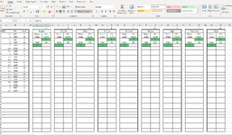
I am wanting to sort data into other columns based on a category shorthand in an adjacent column. I have Estimates in column A and repair order numbers in column B in column C I have a shorthand to indicate who completed the job which can be seen in row 1. What I am wanting to do is automatically have the “est.” number from Colum A show in the “hours” column and the “RO.” Number in column B show in the “list” column under the name of the person who’s shorthand is entered next to it. Also if it is possible I am wanting all the listed numbers to be moved up so that there are no blank spaces between the data points when they show under a name. unfortunaly i am using a work computer

 

[JamesCanale]

Here is something. If you actually want to sort the lists for each guy by EST or RO, that can be done too. Now it's keeping the same order, just binning them.

MrExcelPlayground18.xlsx
	A	B	C	D	E	F	G	H	I	J	K	L	M	N	O	P	Q	R	S	T	U	V	W	X	Y	Z	AA	AB	AC	AD
1						S			T			M			D			H			AK			E			Y			AL
2	EST	RO	Tech		Sparky			Tarrell			Mike			Donnie			Harrison			Akeem			Edgar			Yancarlos			Aldo
3	1.3	4567	D		Hours	RO		Hours	RO		Hours	RO		Hours	RO		Hours	RO		Hours	RO		Hours	RO		Hours	RO		Hours	RO
4	2	3453	M		Week	Count		Week	Count		Week	Count		Week	Count		Week	Count		Week	Count		Week	Count		Week	Count		Week	Count
5	1.6	3461	H			4			0			3			4			2			2			3			2			1
6	2	7357	AK		Total	List		Total	List		Total	List		Total	List		Total	List		Total	List		Total	List		Total	List		Total	List
7	4	2975	S		15536			0			12322			13783			11104			14943			16668			17329			3476
8	1.8	9756	E		4	2975					2	3453		1.3	4567		1.6	3461		2	7357		1.8	9756		1	7453		1.4	3476
9	1.1	2436	D		2.5	2563					2.7	1234		1.1	2436		2.3	7643		1.3	7586		3.5	2345		2	9876
10	1	7453	Y		1.1	7654					1.6	7635		2.5	2345								1	4567
11	2.5	2563	S		1.4	2344								1.7	4435
12	2.3	7643	H
13	1.4	3476	AL
14	2.5	2345	D
15	2.7	1234	M
16	1.1	7654	S
17	1.6	7635	M
18	1.7	4435	D
19	1.3	7586	AK
20	3.5	2345	E
21	2	9876	Y
22	1	4567	E
23	1.4	2344	S
24
25
26
27
Sheet21

Cell Formulas
Range	Formula
F5,AD5,AA5,X5,U5,R5,O5,L5,I5	F5	=IF(E8<>"",ROWS(E8#),0)
E7,AC7,Z7,W7,T7,Q7,N7,K7,H7	E7	=IFERROR(SUM(INDEX(E8#,,2)),0)
E8:F11,AC8:AD8,Z8:AA9,W8:X10,T8:U9,Q8:R9,N8:O11,K8:L10,H8	E8	=IFERROR(FILTER($A$3:$B$45,$C$3:$C$45=F1),"")
Dynamic array formulas.