Automating Time Card Data Collection

[McLaren]

Good morning all. This is quite a bit above my head so I'm hoping someone can help me out. I use a mobile app to log in and out of projects, which then exports out as a csv that I copy into the 2nd sheet of my file like this:

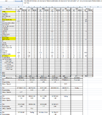
My 1st sheet looks like this:

So I've managed to get the top half of the sheet grouping hours by day/client/customer using SUMIFS, but now I would like to populate the bottom half with Column D and removing the duplicates. So far I have managed to find a formula that works to isolate Rows using Column A:

={INDEX($A$1:$A$200,MATCH("Mon",$A$1:$A$200,0)):INDEX($A$1:$A$200,MAX(IF($A$1:$A$200="Mon",ROW($A$1:$A$200)-MIN(ROW($A$1:$A$200))+1)))}

But now I'm stuck. Any help would be greatly appreciated!

 

[McLaren]

Page 16 bump.

 

[McLaren]

Bump

 

[McLaren]

Figured it out. A bunch of the help came from this video. 1st step was 6 defined names to make dynamic ranges that look at the job(work unit notes) by isolating rows based on the day of the week in the imported sheet('Daily Job Description'). Each name matched the days of the week, Mon, Tue, etc.

=INDEX('Daily Job Description'!$D$2:$D$100,MATCH("Mon",'Daily Job Description'!$A$2:$A$100,0)):INDEX('Daily Job Description'!$D$2:$D$100,MAX(IF('Daily Job Description'!$A$2:$A$100="Mon",ROW('Daily Job Description'!$A$2:$A$100)-MIN(ROW('Daily Job Description'!$A$2:$A$100))+1)))

Then to populate the P/N row under each day

Cell B50:

=IFERROR(INDEX(Mon,MATCH(0,COUNTIF(Mon,"<"&Mon)-SUM(COUNTIF(Mon,B$49:B49)),0)),"")

Cell B54

=IFERROR(INDEX(Mon,MATCH(0,COUNTIF(Mon,"<"&Mon)-SUM(COUNTIF(Mon,B$49:B50)),0)),"")

Cell B58

=IFERROR(INDEX(Mon,MATCH(0,COUNTIF(Mon,"<"&Mon)-SUM(COUNTIF(Mon,B$49:B54)),0)),"")

etc.

Next up to get the number of hours I used a SUMIFS that looks at the P/N cell and adds up all instances within the defined name for the day. To prevent cells showing zeroes it was doubled up with an IF statement. Example of Cell B51:

=IF(SUMIFS('Daily Job Description'!$E$2:$E$100,'Daily Job Description'!$A$2:$A$100,"Mon",'Daily Job Description'!$D$2:$D$100,B50,'Daily Job Description'!$I$2:$I$100,"Program")=0,"",(SUMIFS('Daily Job Description'!$E$2:$E$100,'Daily Job Description'!$A$2:$A$100,"Mon",'Daily Job Description'!$D$2:$D$100,B50,'Daily Job Description'!$I$2:$I$100,"Program")))

Since they wanted Setup and Operate grouped together Cell B52 had to be done a little differently with an array constant:

=IF(SUM(SUMIFS('Daily Job Description'!$E$2:$E$100,'Daily Job Description'!$A$2:$A$100,"Mon",'Daily Job Description'!$D$2:$D$100,B50,'Daily Job Description'!$I$2:$I$100,{"Setup","Run"}))=0,"",SUM(SUMIFS('Daily Job Description'!$E$2:$E$100,'Daily Job Description'!$A$2:$A$100,"Mon",'Daily Job Description'!$D$2:$D$100,B50,'Daily Job Description'!$I$2:$I$100,{"Setup","Run"})))

The only thing it choked on in my initial test was a part number that was just numerals with no letters or dashes. It completely ignored it when populating the bottom half. The workaround for now was adding a rev letter to it.