Average of last 5 nonblank values in row with matching date

MatthewChung

New Member
Joined
Nov 18, 2021
Messages
10
Office Version
  1. 365
Platform
  1. Windows
Hi Everyone!

After spending days and days trying to figure out this problem without any success, I decided to seek further assistance by posting it here. I understand there are some very similar posts which I have been through but it got out of hand very quickly...

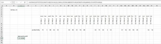
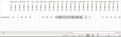
I am working in a table with daily productivity rates and would like to determine the average of the last 5 working days (excluding blanks) based on a moving date. The formula below was what I started with but it included blanks as well which returned an average of 54 when I wanted it to return an average of 60.

=AVERAGE(OFFSET(E9,0,MATCH(B2,F6:AI6,0),1,-5))

As soon as I added additional criteria in the formula below, it returned strange values and became way to difficult for me to understand.

=AVERAGE(OFFSET(E9,0,MATCH(B2,F6:AI6,0),1,SMALL(IF(ISNUMBER(F9:AI9),ROW(F9:AI9)),MIN(5,COUNT(F9:AI9)))))

Any help would be very much appreciated. Thank you!
 

Attachments

  • Average Offset Formula.JPG
    Average Offset Formula.JPG
    141.2 KB · Views: 24

Excel Facts

How to change case of text in Excel?
Use =UPPER() for upper case, =LOWER() for lower case, and =PROPER() for proper case. PROPER won't capitalize second c in Mccartney
cannot manipulate data in a picture. please reload data using xl2bb. See my signature for instructions.
 
Upvote 0
Hi Mathew,

Maybe this setup, then your Workdays header row won't include weekends;

Cell Formulas
RangeFormula
C6C6=TODAY()
G6:AA6G6=WORKDAY($F$6,COLUMNS($G$6:G6))
D11D11=TODAY()-1
D12D12=WORKDAY(D11,-4)
C14C14=AVERAGEIFS($F$9:$AA$9,$F$6:$AA$6,">="&$D$12,$F$6:$AA$6,"<="&$D$11,$F$9:$AA$9,"<>""")

Hi Ras

Thank you for the response. The screenshot I attached was a bad example sorry. Sometimes there will be productivity over the weekend and sometimes there won't. Is there a possible work around for this scenario?
 
Upvote 0
cannot manipulate data in a picture. please reload data using xl2bb. See my signature for instructions.
Hi alan

I managed to get it to work after watching the video.

Book1.xlsx
BCDEFGHIJKLMNOPQRSTUVWXYZAAABACADAEAFAGAHAI
218-Nov-21
3
4
5montuewedthufrisatsunmontuewedthufrisatsunmontuewedthufrisatsunmontuewedthufrisatsunmontue
61-Nov-212-Nov-213-Nov-214-Nov-215-Nov-216-Nov-217-Nov-218-Nov-219-Nov-2110-Nov-2111-Nov-2112-Nov-2113-Nov-2114-Nov-2115-Nov-2116-Nov-2117-Nov-2118-Nov-2119-Nov-2120-Nov-2121-Nov-2122-Nov-2123-Nov-2124-Nov-2125-Nov-2126-Nov-2127-Nov-2128-Nov-2129-Nov-2130-Nov-21
7
8
9productivity711486531438521938461916131317164343205656
10
11
12last work week
1322.14286
Sheet1
Cell Formulas
RangeFormula
C13C13=AVERAGE(OFFSET(E9,0,MATCH(B2,F6:AI6,0),1,SMALL(IF(ISNUMBER(F9:AI9),ROW(F9:AI9)),MIN(5,COUNT(F9:AI9)))))
 
Upvote 0
Can you explain how you come up with 60. When I average the last 5 working days I get 43.6. What am I missing in understanding your needs. Your layout is not conducive to analysis. If you unpivot your data so that it is columnar (normalized) then you can do averages and/or pivot tables which will allow you more flexibility.
Hi alan

For this scenario, I would like to determine the last five cells with values in them starting from 18 November 21 so it would be something like the below / attached image.

18 Nov 21 = 3
17 Nov 21 = 61
16 Nov 21 = 91
15 Nov 21 = 61
12 Nov 21 = 84
 

Attachments

  • Capture.JPG
    Capture.JPG
    86.7 KB · Views: 8
Upvote 0
This works with weekends included

Average of last 5 nonblank values in row with matching date_Matthew Chung.xlsx
CDEFGHIJKLMNOPQRSTUVWXYZAAABACADAEAFAGAHAI
619/11/20211-Nov-212-Nov-213-Nov-214-Nov-215-Nov-216-Nov-217-Nov-218-Nov-219-Nov-2110-Nov-2111-Nov-2112-Nov-2113-Nov-2114-Nov-2115-Nov-2116-Nov-2117-Nov-2118-Nov-2119-Nov-2120-Nov-2121-Nov-2122-Nov-2123-Nov-2124-Nov-2125-Nov-2126-Nov-2127-Nov-2128-Nov-2129-Nov-2130-Nov-21
7
8
9productivity711486531438521938461916131317164343205656
10
11Yesterday18/11/2021
125 days Prior12/11/2021
13Last Week
1460
Sheet1
Cell Formulas
RangeFormula
C6C6=TODAY()
D11D11=TODAY()-1
D12D12=WORKDAY(D11,-4)
C14C14=AVERAGEIFS($F$9:$AI$9,$F$6:$AI$6,">="&$D$12,$F$6:$AI$6,"<="&$D$11,$F$9:$AI$9,"<>""")
 
Upvote 0
Hi RasGhul

That ALMOST worked! I put some values in the Saturday and Sunday column and your formula skips these days.

Book1.xlsx
ABCDEFGHIJKLMNOPQRSTUVWXYZAAABACADAEAFAGAHAIAJ
1
218-Nov-21
3
4
5montuewedthufrisatsunmontuewedthufrisatsunmontuewedthufrisatsunmontuewedthufrisatsunmontue
61-Nov-212-Nov-213-Nov-214-Nov-215-Nov-216-Nov-217-Nov-218-Nov-219-Nov-2110-Nov-2111-Nov-2112-Nov-2113-Nov-2114-Nov-2115-Nov-2116-Nov-2117-Nov-2118-Nov-2119-Nov-2120-Nov-2121-Nov-2122-Nov-2123-Nov-2124-Nov-2125-Nov-2126-Nov-2127-Nov-2128-Nov-2129-Nov-2130-Nov-21
7
8
9productivity711486531438521938415619161313917164343205656
10
11
12
13
14
15last work week57
16
17
Sheet1
Cell Formulas
RangeFormula
D15D15=AVERAGEIFS($F$9:$AI$9,$F$6:$AI$6,">="&B2-5,$F$6:$AI$6,"<="&B2-1,$F$9:$AI$9,"<>""")
 
Upvote 0

Forum statistics

Threads
1,215,360
Messages
6,124,489
Members
449,166
Latest member
hokjock

We've detected that you are using an adblocker.

We have a great community of people providing Excel help here, but the hosting costs are enormous. You can help keep this site running by allowing ads on MrExcel.com.
Allow Ads at MrExcel

Which adblocker are you using?

Disable AdBlock

Follow these easy steps to disable AdBlock

1)Click on the icon in the browser’s toolbar.
2)Click on the icon in the browser’s toolbar.
2)Click on the "Pause on this site" option.
Go back

Disable AdBlock Plus

Follow these easy steps to disable AdBlock Plus

1)Click on the icon in the browser’s toolbar.
2)Click on the toggle to disable it for "mrexcel.com".
Go back

Disable uBlock Origin

Follow these easy steps to disable uBlock Origin

1)Click on the icon in the browser’s toolbar.
2)Click on the "Power" button.
3)Click on the "Refresh" button.
Go back

Disable uBlock

Follow these easy steps to disable uBlock

1)Click on the icon in the browser’s toolbar.
2)Click on the "Power" button.
3)Click on the "Refresh" button.
Go back
Back
Top