Calculate tangent-present on graph and in table

[TorrO]

Hi

Case:
I have tried to make tangents based on pulse min/max per interval, I don't find the solution.
Also add tangent to graph is nothing I manage to understand.

Question:
Add tangents to a graph based on min and max values for each drag and brake, also add a table for tangent angles.


I have this graph, 33 minute workout, each second has a pulse reading.

Data

What I would like to present is a tangent with a angle, something like this:

And also make a table representing all intervals like this, data set you can download further down.

Inteval - tangent angle
number
1 30 deg
2 -84 deg
3 34 deg
4 -78 deg
....
21 40 deg -80 deg -> as many drags there is in workout data, presented in column J=Interval number

Data is here

Thanks up front

 

[Anthony47]

Probably something can be done by working on the data serie values; if you can share a demo workbook with real data maybe we can work on it

 

[TorrO]

Probably something can be done by working on the data serie values; if you can share a demo workbook with real data maybe we can work on it

Hi

thanks for answer.
Sorry for late answer.
workbook here

 

[Anthony47]

Something can be done, assuming that minimums and maximums follow each other with a regular rhythm; but the user need to provide few critical parametres, and the result should be checked to be sure that there aren't severe errors.

Let's use a User Function to get the coordinates of the peaks (min and max). I called it "SerieInfoTabl" and corresponds to the following code:

Function SerieInfoTabl(ByVal m1Point As Long, ByVal m2Point, ByVal ePoint As Long) As Variant
Dim aChart As Chart, yArea As String, mySplit
Dim PulseForm As String, SRSplit, oInd As Long
Dim oArr()
Dim MinY As Single, MinX As Long, MaxY As Single, MaxX As Long
'
Set aChart = ActiveSheet.ChartObjects(1).Chart
'
ReDim oArr(1 To 2, 0 To 4)
PulseForm = aChart.SeriesCollection("Pulse").Formula
mySplit = Split(PulseForm, ",", , vbTextCompare)
yArea = mySplit(UBound(mySplit) - 1)
oInd = 1
For j = 1 To 50
    span = (m2Point - m1Point)
    'Debug.Print span
    For i = 0 To 1
        If i = 0 Then bPoint = m1Point Else bPoint = m2Point
        SRSplit = Split(Replace(yArea, "'", "", , , vbTextCompare), "!", , vbTextCompare)
        MinY = Application.WorksheetFunction.Min(Sheets(SRSplit(0)).Range(SRSplit(1)).Cells(1, 1).Offset(bPoint - span / 4, 0).Resize(span / 2, 1))
        'Debug.Print "MinY = " & MinY, Sheets(SRSplit(0)).Range(SRSplit(1)).Cells(1, 1).Offset(bPoint - span / 4, 0).Resize(span / 2, 1).Address(0, 0); ""
        MinX = Application.Match(MinY, Sheets(SRSplit(0)).Range(SRSplit(1)).Cells(1, 1).Offset(bPoint - span / 4, 0).Resize(span / 2, 1), False) + bPoint - span / 4
        MaxY = Application.WorksheetFunction.Max(Sheets(SRSplit(0)).Range(SRSplit(1)).Cells(1, 1).Offset(bPoint + span / 6, 0).Resize(span / 2, 1))
        'Debug.Print "MaxY=" & MaxY, Sheets(SRSplit(0)).Range(SRSplit(1)).Cells(1, 1).Offset(bPoint + span / 6, 0).Resize(span / 2, 1).Address(0, 0)
        MaxX = Application.Match(MaxY, Sheets(SRSplit(0)).Range(SRSplit(1)).Cells(1, 1).Offset(bPoint + span / 6, 0).Resize(span / 2, 1), False) + bPoint + span / 6
        oArr(1, oInd + 0 + i * 2) = MinX: oArr(2, oInd + 0 + i * 2) = MinY: oArr(1, oInd + 1 + i * 2) = MaxX: oArr(2, oInd + 1 + i * 2) = MaxY
    Next i
    oInd = oInd + 4
    m1Point = MinX
    m2Point = m1Point + (MaxX - MinX) * 2
    If m2Point > ePoint Then Exit For
    ReDim Preserve oArr(1 To 2, 0 To UBound(oArr, 2) + 2)
    oInd = oInd - 2
Next j
oArr(1, 0) = j * 2 + 2
If Parent.Caller.Columns.Count > UBound(oArr, 2) Then
    ReDim Preserve oArr(1 To 2, 0 To Parent.Caller.Columns.Count)
ElseIf Parent.Caller.Columns.Count < UBound(oArr, 2) Then
    oArr(2, 0) = (UBound(oArr, 2) - Parent.Caller.Columns.Count) & "##"
End If
'Debug.Print "J=" & j
SerieInfoTabl = oArr
End Function

It requires 3 parametres:
-the X (horizontal) position of the first Minimum to consider
-the X position of the second Minimum
-the X position of the last Minimum to consider
(all these info can be provided with a certain level of tolerance)

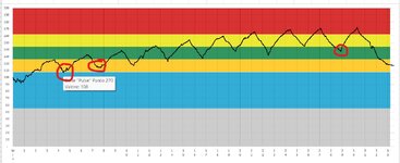
Using the file you provided, I have noted the 3 highlighted coordinates (see first image): setting the mouse near the points I got the following X positions:
270; 463; 1750
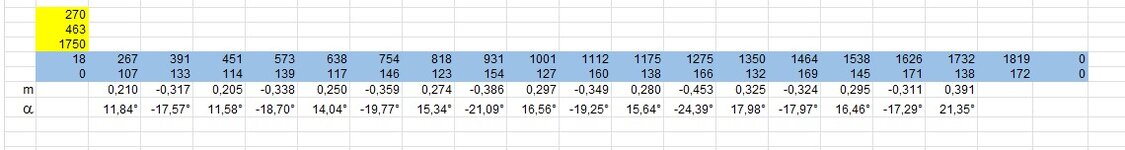
I loaded these values in cells W20-W21-W22 (see the second image)

With these parametres we are ready to get the best guess of the peaks via the Function SerieInfoTabl, using in W23 the following formula:

=SerieInfoTabl(W20,W21,W22)

It is an array formula and need to be inserted into an area of 2 Rows * N Columns:
-Select W23:AP24 (I'll explain later how setting the area)
-Set the given formula into the Formula bar
-Confirm the formula using the combination Contr-Shift-Enter, not Enter alone

This should return a sequence or Paired cells (vertical paired) that contains the X (first row) and Y (second row) of the first Minimum; the X and the Y of the first Maximun; the X and the Y of the second Minimum; and so on until the latest X to consider (1750, set in W22, in my example)

See the second image (the yellow area are the 3 parametres; the blue area are the values returned by the formula)

The first column of the returned result contains "service information":
-the first Row specify how many nodes are returned by the function (18, in my example)
-the second Row contains either 0, if the formula has been entered in an area enough wide to contains all the results; or N## if the area is not wide enough, and N will state how many columns are missing. In this second hypotesis, if you want to extend the formula on additional columns:
-Select the current Area; extend the selection for as many columns you need; press F2 (edit formula), confirm using Contr-Shift-Enter

In case you set the formula in more columns than those that are necessary, 0 will be used to fill the unused columns

So now we have X1,Y1 of the first Minumum, X2,Y2 of the first Maximum
We can now calculate the "slope" of the line passing from the two pairs of coordinates using the formula
m = (Y2-Y1)/(X2-X1)
Translated to Excel: in X25 I used the formula

=(Y24-X24)/(Y23-X23)

Finally we can calculate the angle of this first line using
alpha = ATAN(slope)

Translated in Excel, with results in Degres, in X26 I used the formula

=DEGREES(ATAN(X25))

Now copy X25:X26 to the right for as many nodes you have

This is shown in the folllowing XL2BB minisheet

byTORRO-MrEX_PulseFitReportv1-mRX_C21031.xlsm
	V	W	X	Y	Z	AA	AB	AC	AD	AE	AF	AG	AH	AI	AJ	AK	AL	AM	AN	AO	AP	AQ
18
19
20		270
21		463
22		1750
23		18	267	391	451	573	638	754	818	931	1001	1112	1175	1275	1350	1464	1538	1626	1732	1819	0
24		0	107	133	114	139	117	146	123	154	127	160	138	166	132	169	145	171	138	172	0
25	m		0,210	-0,317	0,205	-0,338	0,250	-0,359	0,274	-0,386	0,297	-0,349	0,280	-0,453	0,325	-0,324	0,295	-0,311	0,391
26	a		11,84°	-17,57°	11,58°	-18,70°	14,04°	-19,77°	15,34°	-21,09°	16,56°	-19,25°	15,64°	-24,39°	17,98°	-17,97°	16,46°	-17,29°	21,35°
27
Presentation

Cell Formulas
Range	Formula
W23:AP24	W23	=SerieInfoTabl(W20,W21,W22)
X25:AN25	X25	=(Y24-X24)/(Y23-X23)
X26:AN26	X26	=DEGREES(ATAN(X25))
Press CTRL+SHIFT+ENTER to enter array formulas surrounded with curly braces.

A couple of final notices:
-the function works by analyzing the source data of the serie named "Pulse" of graph #1 of the active sheet
-the users that have an Excel version that support Dynamic Array may insert the formula that uses SerieInfoTabl in a single cell and its results will expand for 2 rows * N columns (N as needed)

HTH...

 

[TorrO]

Hi Anthony47

Thanks for your effort.
I will try to implement this code, it will take some time due to heavy work load.

You will hear more from me.

Thanks!