Cannot change date format on Pivot Chart created using Power Pivot

JollyRoger01

New Member
Joined
Jun 1, 2021
Messages
12
Office Version
  1. 365
  2. 2016
Platform
  1. Windows
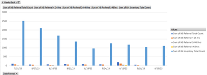
I have been through hundreds of web pages looking for a solution to this and have not been able to find a solution. Apparently, if creating a Pivot Table and subsequent Pivot Chart from the Data Model, I need to ensure that there are no 0's or blanks in the date column if I want to access the Number Format button when left clicking on the date field in the Field Settings. I have gone through my data over and over and everything is fine, I have no missing values. I can change the format of the pivot table fine using the normal number format dropdown from the ribbon. But the axis of the chart refuses to change. I have tried changing the format in Power Pivot, through the Format Axis bit, using the dropdown on the ribbon... Nothing works!

Could someone please help me and change the number format in the workbook below to DD MMM YYYY?


Excel Facts

Copy a format multiple times
Select a formatted range. Double-click the Format Painter (left side of Home tab). You can paste formatting multiple times. Esc to stop
Can you reshare the workbook allowing anyone with the link to open it. I suspect you can't do that using Sharepoint so if you can try Google drive, OneDrive, Dropbox or one of the other sharing platforms.

Some considerations:
Did you load the data into the data model ? If so what is the columns Data Type set to ?
If you have a table what do you get if you filter the offending column for blanks or text or Errors such as #N/A ?
Also with no filters applied to the Pivot, go to the date filter drop down on the pivot and look for the items that appear right at the beggining of the list and right at the end of the list.
Dates out of order will be text and blanks and #errors will also float to the top or bottom.
 
Upvote 0
Try removing all date columns from all pivots, make sure the format of the date column is as needed in the model. Go to the model and add a calc column (column:=1 is fine). This forces a change to the model and should refresh the cache. For good measure, go back to excel and refresh all. Go to a new page and insert a new Pivot.
if that doesn’t work, then 🤷‍♂️
 
Upvote 0
Add Column in your Power Pivot Table. Use FORMAT('Date'[Date],"DD/MMM/YYYY")
Use this new field for your pivot table X axis.
This has been the only solution that I've found.
 

Attachments

  • Screenshot 2023-09-26 133043.png
    Screenshot 2023-09-26 133043.png
    18.1 KB · Views: 64
Upvote 0

Forum statistics

Threads
1,215,643
Messages
6,125,990
Members
449,278
Latest member
MOMOBI

We've detected that you are using an adblocker.

We have a great community of people providing Excel help here, but the hosting costs are enormous. You can help keep this site running by allowing ads on MrExcel.com.
Allow Ads at MrExcel

Which adblocker are you using?

Disable AdBlock

Follow these easy steps to disable AdBlock

1)Click on the icon in the browser’s toolbar.
2)Click on the icon in the browser’s toolbar.
2)Click on the "Pause on this site" option.
Go back

Disable AdBlock Plus

Follow these easy steps to disable AdBlock Plus

1)Click on the icon in the browser’s toolbar.
2)Click on the toggle to disable it for "mrexcel.com".
Go back

Disable uBlock Origin

Follow these easy steps to disable uBlock Origin

1)Click on the icon in the browser’s toolbar.
2)Click on the "Power" button.
3)Click on the "Refresh" button.
Go back

Disable uBlock

Follow these easy steps to disable uBlock

1)Click on the icon in the browser’s toolbar.
2)Click on the "Power" button.
3)Click on the "Refresh" button.
Go back
Back
Top