Change in output generated by a macro

Valentino

Board Regular
Joined
Mar 28, 2010
Messages
105
Hi everyone,

in another thread, @johnnyL has helped me tremendously by developing a code which regularly checks whether certain conditions in a spreadsheet have been fulfilled.
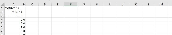
Every 10 minutes, the macro writes the outcome of these checks to a separate outputsheet, which alerts me to changes in conditions.
What i still would like to achieve, is to change the current notification generated by this macro.
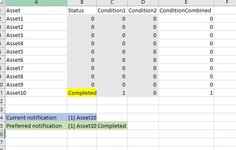
- Current notification: "(1) Asset10" --> (indicating that Asset10 changed from "0" to "1", see blue cell in picture below)
- preferred notification: "(1) Asset10 Completed" --> (so add the value from column B in Sheet1 highlighted in yellow to the notification).

Below please find the code that i have been working with and attached a picture of Sheet1 in the workbook containing the value to be added (in yellow) .

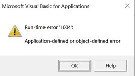
I have been trying to adjust the code myself based on some solutions i found on this forum and elsewhere, but have struggled as after I've changed the code is bugged (my inexperience) :(
Would someone be able to help me to adjust the code?

Many thanks for thoughts!

Valentino

VBA Code:
Private Sub Worksheet_Calculate()
'
'   V1.2
'   1st 10 minute refresh will create the destination if it doesn't exist & will save the Formula column results to create a base line to compare to.
'   All other 10 minute refreshes will compare the current formula column to the previous formula column and display the row #s that changed to '1' or '-1'.
'
'   Check the lines at the top of the script that end with ' <---
'       Those lines are the lines that may need to be changed to reflect your particular setup.
'
'
    Dim FormulaStartRow                 As Long, LastRowAssetColummn    As Long
    Dim DestinationSheet                As String
    Dim AssetColumn                     As String, FormulaColumn        As String
    Dim wsDestination                   As Worksheet, wsSource          As Worksheet
'
    DestinationSheet = "TenMinuteUpdates"                           ' <--- Set this to the name of the sheet to store 10 minute results into
    Set wsSource = ThisWorkbook.Sheets("Sheet1")                    ' <--- Set this to the sheetname that has the '1's & '0's
'
      FormulaColumn = "E"                                           ' <--- Set this to the formula Column letter
    FormulaStartRow = 2                                             ' <--- Set this to the start row of formulas in the FormulaColumn
       AssetColumn = "A"                                            ' <--- Set this to the Asset Column letter, this column is used to determine last row
'
    LastRowAssetColummn = wsSource.Range(AssetColumn & Rows.Count).End(xlUp).Row ' Determine last row of data
'
    If Application.CountIf(wsSource.Range(FormulaColumn & FormulaStartRow & _
            ":" & FormulaColumn & LastRowAssetColummn), "1") > 0 Or _
            Application.CountIf(wsSource.Range(FormulaColumn & FormulaStartRow & _
            ":" & FormulaColumn & LastRowAssetColummn), "-1") > 0 Then  ' If the range contains any value of 1 or -1 then ...
'
        Dim DestinationSheetExists      As Boolean
        Dim FormulaColumnRow            As Long, OutputArrayRow As Long
        Dim LastDestinationColumnNumber As Long
        Dim RowOffset                   As Long
        Dim AssetColumnArray            As Variant, FormulaColumnArray          As Variant
        Dim OutputArray                 As Variant, PreviousFormulaResultArray  As Variant
'
        On Error Resume Next                                        '   Bypass error generated in next line if sheet does not exist
        Set wsDestination = ThisWorkbook.Sheets(DestinationSheet)   '   Assign DestinationSheet to wsDestination
        On Error GoTo 0                                             '   Turn Excel error handling back on
'
        If Not wsDestination Is Nothing Then DestinationSheetExists = True      '   Check to see if the DestinationSheet exists
'
' Create DestinationSheet if it doesn't exist
        If DestinationSheetExists = False Then                                  '   If DestinationSheet does not exist then ...
            ThisWorkbook.Sheets.Add(After:=wsSource).Name = DestinationSheet    '       Create the DestinationSheet after the Source sheet
            Set wsDestination = ThisWorkbook.Sheets(DestinationSheet)           '       Assign the DestinationSheet to wsDestination
        End If
'
' Save Assets into array
        AssetColumnArray = wsSource.Range(AssetColumn & _
                FormulaStartRow & ":" & AssetColumn & _
                LastRowAssetColummn)                                '   Save the values of the Asset Column range into the 2D 1 based AssetColumnArray RC
'
' Save formulas into array
        FormulaColumnArray = wsSource.Range(FormulaColumn & _
                FormulaStartRow & ":" & FormulaColumn & _
                LastRowAssetColummn)                                '   Save the values of the formula Column range into the 2D 1 based FormulaColumnArray RC
'
        ReDim OutputArray(1 To UBound(FormulaColumnArray))          '   Establish # of rows in 1D 1 based OutputArray
'
' Create Saved formula result column on DestinationSheet
        If wsDestination.Range("A1") = vbNullString Then
            wsDestination.Range("A1") = Date                        '   Display the Date on DestinationSheet
            wsDestination.Range("A2") = Time()                      '   Display the Time on DestinationSheet
            wsDestination.Range("A3") = "------------------"        '   Display spacer line on DestinationSheet
'
            wsDestination.Range("A4").Resize(UBound(FormulaColumnArray)) = _
                FormulaColumnArray                                  '   Display results to DestinationSheet
'
            wsDestination.UsedRange.EntireColumn.AutoFit            '   Autofit all of the columns
'
            GoTo SubExit
        End If
'
' Load previous formula results into array
        PreviousFormulaResultArray = wsDestination.Range("A4:A" & _
                wsDestination.Range("A" & Rows.Count).End(xlUp).Row)    '   Load previous formula results into PreviousFormulaResultArray
'
        OutputArrayRow = 0                                          '   Initialize OutputArrayRow to zero
        RowOffset = FormulaStartRow - LBound(FormulaColumnArray)    '   Determine Row difference between FormulaStartRow and start row of FormulaColumnArray
'
'-------------------------------------------------------------------
'
        For FormulaColumnRow = 1 To UBound(FormulaColumnArray, 1)   '   Loop through the FormulaColumnArray to check for '1's & '-1's
            If FormulaColumnArray(FormulaColumnRow, 1) = "1" Or _
                    FormulaColumnArray(FormulaColumnRow, 1) = "-1" Then '       If a '1' or '-1' is found then ...
                If PreviousFormulaResultArray(FormulaColumnRow, 1) = 0 Then '       If previous value was '0' then ...
                    OutputArrayRow = OutputArrayRow + 1                 '           Increment OutputArrayRow
'
                    OutputArray(OutputArrayRow) = "(" & _
                            FormulaColumnArray(FormulaColumnRow, 1) & _
                            ") " & AssetColumnArray(FormulaColumnRow, 1)    '           Save the changed to value & Asset into OutputArray
                End If
            End If
        Next                                                        '   Loop Back
'
        LastDestinationColumnNumber = wsDestination.Cells.Find("*", _
                , xlFormulas, , xlByColumns, xlPrevious).Column     '   Get last Column Number used in the DestinationSheet
'
        wsDestination.Cells(1, LastDestinationColumnNumber + 1) = Date      '   Display the Date on DestinationSheet
        wsDestination.Cells(2, LastDestinationColumnNumber + 1) = Time()    '   Display the Time on DestinationSheet
        wsDestination.Cells(3, LastDestinationColumnNumber + 1) = "------------------"  '   Display spacer line on DestinationSheet
'
        wsDestination.Cells(4, LastDestinationColumnNumber _
                + 1).Resize(UBound(OutputArray)) = _
                Application.Transpose(OutputArray)                  '   Display results to DestinationSheet
'
'Save current formula results to the DestinationSheet
        wsDestination.Range("A1") = Date                            '   Display the Date on DestinationSheet
        wsDestination.Range("A2") = Time()                          '   Display the Time on DestinationSheet
        wsDestination.Range("A3") = "------------------"            '   Display spacer line on DestinationSheet
'
        wsDestination.Range("A4").Resize(UBound(FormulaColumnArray)) = _
            FormulaColumnArray                                      '   Display results to DestinationSheet
'
        wsDestination.UsedRange.EntireColumn.AutoFit                '   Autofit all of the columns
    End If
'
'-------------------------------------------------------------------
'
SubExit:
End Sub
 

Attachments

  • Pic7.JPG
    Pic7.JPG
    41.7 KB · Views: 12
Also, you didn't answer if you had deleted the destination sheet prior to trying the newest code. You would want to delete that sheet prior to running the code so you don't start with a 'filled' destination sheet.
 
Upvote 0

Excel Facts

Which Excel functions can ignore hidden rows?
The SUBTOTAL and AGGREGATE functions ignore hidden rows. AGGREGATE can also exclude error cells and more.
Also, you didn't answer if you had deleted the destination sheet prior to trying the newest code. You would want to delete that sheet prior to running the code so you don't start with a 'filled' destination sheet.
Johnny, indeed i later thought of deleting the destination sheet, but still the error recurred...same part of the code when i debug, and also mentions 16384.
See attached a screenshot of the outputsheet, as you can see only the first columns are used, rest is empty! In fact, i would expect some more columns to be used as some assets changed from "0" to "1" or "-1" which it did not detect...:( (version 2.1 does this very well therefore still my favorite!)
 

Attachments

  • Pic17.JPG
    Pic17.JPG
    39.4 KB · Views: 3
Upvote 0
Without actually being able to run the script, I honestly have no clue why your destination sheet columns are getting maxed out.

How quickly does that error occur after starting the script?
 
Upvote 0
Without actually being able to run the script, I honestly have no clue why your destination sheet columns are getting maxed out.

How quickly does that error occur after starting the script?
Strange indeed! I opened the file, deleted the destination sheet and error happened after the second 10min refresh of the webquery. If it helps i could share the workbook with the error, but given that this version also seems to miss some asset changes perhaps we should stick with v2.1 and leave out the formula feature i had in mind and which caused the runtime error. Its still a very nice result which will greatly help!!
 
Upvote 0
I guess you should stick with what works.
Indeed! As said, it works well and i will use coming weeks to test and refine, and will report back. I marked post #10 of this thread as solution. Many thanks to you for all the efforts! :)
 
Upvote 0
You are welcome.
@johnnyL , Others,
in post 10 of this thread a code was created, which has helped me a lot.
As a final step in this project, i'd like to add some functionality (some very simple copy paste actions), which i have created by recording a macro and which i'd like to be executed everytime the macro has run. See the additional code below.
I've tried to paste in the beginning and end of the original code, but then i got a runtime error 1004 message (see attached picture). I must be doing something wrong... i googled this error and could be related to some missing (sheet) names?

Could anyone show me please how to integrate the additional code into the original code?
If not possible, would there be another way to trigger the other macro so that it runs each time the original macro runs?

many thanks!
Valentino

Additional code:
SQL:
 Sheets("Historical").Select
    Range("A2:D2").Select
    Range(Selection, Selection.End(xlDown)).Select
    Selection.Copy
    Range("I2").Select
    Selection.PasteSpecial Paste:=xlPasteValues, Operation:=xlNone, SkipBlanks _
        :=False, Transpose:=False
    Range("T2").Select
    Range(Selection, Selection.End(xlToRight)).Select
    Range(Selection, Selection.End(xlDown)).Select
    Application.CutCopyMode = False
    Selection.Copy
    Range("a1").Select

To be integrated in original code:
SQL:
Private Sub Worksheet_Calculate()
'
'   V2.1
'
'   1st 10 minute refresh will create the DestinationSheet if it doesn't exist & will save the conditions column results to create a base line to compare to.
'   All other 10 minute refreshes will compare the current condition columns to the previous condition columns and display the Assets that had
'       conditions changed to '1' or '-1'
'
'   Check the lines at the top of the script that end with ' <---
'       Those lines are the lines that may need to be changed to reflect your particular setup.
'
    Dim CurrentConditionsStartRow               As Long, LastRowAssetColummn                As Long
    Dim CurrentConditionsRange                  As Range
    Dim DestinationSheet                        As String
    Dim AssetColumn                             As String, StatusColumn                     As String
    Dim FirstConditionColumn                    As String, SecondConditionColumn            As String
    Dim ConditionsCombinedColumn                As String
    Dim wsDestination                           As Worksheet, wsSource                      As Worksheet
'
    DestinationSheet = "TenMinuteUpdates"                               ' <--- Set this to the name of the sheet to store 10 minute results into
    Set wsSource = ThisWorkbook.Sheets("Sheet1")                        ' <--- Set this to the sheetname that has the '1's & '0's
'
                  AssetColumn = "A"                                     ' <--- Set this to the Asset Column letter, this column is used to determine last row
                 StatusColumn = "B"                                     ' <--- Set this to the column letter of the StatusColumn
         FirstConditionColumn = "C"                                     ' <--- Set this to the column letter of the first condition
        SecondConditionColumn = "D"                                     ' <--- Set this to the column letter of the second condition
     ConditionsCombinedColumn = "E"                                     ' <--- Set this to the column letter of the ConditionsCombined Column
    CurrentConditionsStartRow = 2                                       ' <--- Set this to the start row of CurrentConditions
'
    LastRowAssetColummn = wsSource.Range(AssetColumn & _
            Rows.Count).End(xlUp).Row                                   ' Determine last row of data
'
    Set CurrentConditionsRange = wsSource.Range(FirstConditionColumn & _
            CurrentConditionsStartRow & ":" & SecondConditionColumn & _
            LastRowAssetColummn)                                        ' Establish the ConditionsRange
'
    If Application.CountIf(CurrentConditionsRange, "1") > 0 Or _
            Application.CountIf(CurrentConditionsRange, "-1") > 0 Then         ' If the ConditionsRange contains any value of 1 or -1 then ...
'
        Dim ArrayRowIncremented                 As Boolean, DestinationSheetExists          As Boolean
        Dim ConditionsColumnColumn              As Long, ConditionsColumnRow                As Long
        Dim CurrentConditionValue               As Long
        Dim LastDestinationColumnNumber         As Long
        Dim OutputArrayRow                      As Long
'
        Dim AssetColumnArray                    As Variant, CurrentConditionsArray          As Variant
        Dim DateTimeArray(1 To 2)               As Variant
        Dim PreviousConditionsArray             As Variant, PreviousHeadingsArray(1 To 3)   As Variant
        Dim OutputArray                         As Variant, SourceArray                     As Variant
'
        On Error Resume Next                                                '   Bypass error generated in next line if sheet does not exist
        Set wsDestination = ThisWorkbook.Sheets(DestinationSheet)           '   Assign DestinationSheet to wsDestination
        On Error GoTo 0                                                     '   Turn Excel error handling back on
'
        If Not wsDestination Is Nothing Then DestinationSheetExists = True  '   Check to see if the DestinationSheet exists
'
' Create DestinationSheet if it doesn't exist
        If DestinationSheetExists = False Then                                  '   If DestinationSheet does not exist then ...
            ThisWorkbook.Sheets.Add(after:=wsSource).Name = DestinationSheet    '       Create the DestinationSheet after the Source sheet
            Set wsDestination = ThisWorkbook.Sheets(DestinationSheet)           '       Assign the DestinationSheet to wsDestination
        End If
'
' Load current Conditions into array
        CurrentConditionsArray = CurrentConditionsRange                         '   Load the values of the Condition Columns range into the 2D 1 based
'                                                                               '           ConditionsArray RC
        ReDim OutputArray(1 To UBound(CurrentConditionsArray))                  '   Establish # of rows in 1D 1 based OutputArray
'
        SourceArray = wsSource.Range(AssetColumn & CurrentConditionsStartRow & _
                ":" & ConditionsCombinedColumn & LastRowAssetColummn)           '   Load all source values into SourceArray
'
' Create Saved conditions result columns on DestinationSheet if they haven't been created yet
        If wsDestination.Range("A1") = vbNullString Then                        '   If previous conditions have not been saved then ...
            PreviousHeadingsArray(1) = Date                                     '       Save Date into PreviousHeadingsArray
            PreviousHeadingsArray(2) = Time()                                   '       Save Time into PreviousHeadingsArray
            PreviousHeadingsArray(3) = "------------------"                     '       Save space line into PreviousHeadingsArray
            wsDestination.Range("A1").Resize(UBound(PreviousHeadingsArray, 1)) _
                    = Application.Transpose(PreviousHeadingsArray)              '       Save PreviousHeadingsArray to destination sheet
'
            wsDestination.Range("A4").Resize(UBound(CurrentConditionsArray, 1), _
                    UBound(CurrentConditionsArray, 2)) = CurrentConditionsArray '       Display CurrentConditionsArray to DestinationSheet
'
            wsDestination.UsedRange.EntireColumn.AutoFit                        '       Autofit all of the columns
'
            GoTo SubExit                                                        '       Exit this subroutine
        End If
'
' Load previous conditions results into array
        PreviousConditionsArray = wsDestination.Range("A4:B" & _
                wsDestination.Range("A" & Rows.Count).End(xlUp).Row)            '   Load previous conditions results into PreviousConditionsArray
'                                                                               '           AssetColumnArray RC
'-------------------------------------------------------------------
'
' Find and save changes from zero
        OutputArrayRow = 0                                                      '   Initialize OutputArrayRow to zero
'
        For ConditionsColumnRow = 1 To UBound(CurrentConditionsArray, 1)        '   Loop through the CurrentConditionsArray rows to check for '1's & '-1's
            For ConditionsColumnColumn = 1 To UBound(CurrentConditionsArray, 2) '       Loop through the CurrentConditionsArray columns to check for '1's & '-1's
'
                CurrentConditionValue = CurrentConditionsArray(ConditionsColumnRow, _
                        ConditionsColumnColumn)                                 '           Get the CurrentConditionValue
'
                If CurrentConditionValue = "1" Or CurrentConditionValue = "-1" Then '           If a '1' or '-1' is found then ...
'
                    If PreviousConditionsArray(ConditionsColumnRow, _
                            ConditionsColumnColumn) = 0 Then                    '               If previous value was '0' then ...
                        If ArrayRowIncremented = False Then                     '                   If we haven't already incremented OutputArrayRow then ...
                            OutputArrayRow = OutputArrayRow + 1                 '                       Increment OutputArrayRow
                            ArrayRowIncremented = True                          '                       Set ArrayRowIncremented flag = True
                        End If
'
                        If OutputArray(OutputArrayRow) = vbNullString Then      '                   If OutputArray cell is blank then ...
                            OutputArray(OutputArrayRow) = "(" & _
                            SourceArray(ConditionsColumnRow, 5) & ") " & _
                            SourceArray(ConditionsColumnRow, 1) & " " & _
                            SourceArray(ConditionsColumnRow, 2)                 '                       Save desired result to OutputArray
                        End If
                    End If
                End If
            Next                                                                '       Loop Back
'
            ArrayRowIncremented = False                                         '       Reset the ArrayRowIncremented to False
        Next                                                                    '   Loop Back
'
'-------------------------------------------------------------------
'
' Save found changes to the DestinationSheet
        LastDestinationColumnNumber = wsDestination.Cells.Find("*", _
                , xlFormulas, , xlByColumns, xlPrevious).Column                 '   Get last Column Number used in the DestinationSheet
'
        DateTimeArray(1) = Date
        DateTimeArray(2) = Time()
        wsDestination.Cells(1, LastDestinationColumnNumber + _
                1).Resize(UBound(DateTimeArray, 1)) = _
                Application.Transpose(DateTimeArray)                            '   Display Date & Time to Destination sheet
'
        wsDestination.Cells(4, LastDestinationColumnNumber _
                + 1).Resize(UBound(OutputArray)) = _
                Application.Transpose(OutputArray)                              '   Display results to DestinationSheet
'
'-------------------------------------------------------------------
'
'Save ConditionsArray to the DestinationSheet
        wsDestination.Range("A1").Resize(UBound(DateTimeArray, 1)) _
                    = Application.Transpose(DateTimeArray)                      '   Display Date & Time to destination sheet
'
        wsDestination.Range("A4").Resize(UBound(CurrentConditionsArray, 1), _
                UBound(CurrentConditionsArray, 2)) = CurrentConditionsArray     '   Display results to DestinationSheet
'
        wsDestination.UsedRange.EntireColumn.AutoFit                            '   Autofit all of the columns
    End If
'
'-------------------------------------------------------------------
'
SubExit:
End Sub
 

Attachments

  • Pic18.JPG
    Pic18.JPG
    22.8 KB · Views: 3
Upvote 0
It looks like you left out some of your additional code at the bottom of it.
 
Upvote 0
It looks like you left out some of your additional code at the bottom of it.
Hi Johnny,

thanks for the reply!!
Indeed, it seems the code was not complete, it was a bit shorter version which i tried to avoid the error.
The original code as below is a bit longer, but i get the same message if i use either of them.

Why would it not be possible to integrate this additional code in the original?

thanks!
Valentino

SQL:
Sub CopyHistoric()
'
' CopyHistoric Macro
'

'
    Sheets("Historical").Select
    Range("A2:D2").Select
    Range(Selection, Selection.End(xlDown)).Select
    Selection.Copy
    Range("I2").Select
    Selection.PasteSpecial Paste:=xlPasteValues, Operation:=xlNone, SkipBlanks _
        :=False, Transpose:=False
    Range("T2").Select
    Range(Selection, Selection.End(xlToRight)).Select
    Range(Selection, Selection.End(xlDown)).Select
    Application.CutCopyMode = False
    Selection.Copy
    ActiveWindow.LargeScroll ToRight:=-1
    ActiveWindow.LargeScroll Down:=-5
    Range("A2").Select
    Selection.PasteSpecial Paste:=xlPasteValues, Operation:=xlNone, SkipBlanks _
        :=False, Transpose:=False
    Sheets("Daily").Select
    Range("C2:E2").Select
    Range(Selection, Selection.End(xlDown)).Select
    Application.CutCopyMode = False
    Selection.Copy
    Sheets("Historical").Select
    Range("T2").Select
    ActiveWindow.SmallScroll ToRight:=4
    Selection.PasteSpecial Paste:=xlPasteValues, Operation:=xlNone, SkipBlanks _
        :=False, Transpose:=False
    Sheets("Daily").Select
    ActiveWindow.SmallScroll ToRight:=6
    Range("R2").Select
    Range(Selection, Selection.End(xlDown)).Select
    Application.CutCopyMode = False
    Selection.Copy
    Sheets("Historical").Select
    Range("W2").Select
    Selection.PasteSpecial Paste:=xlPasteValues, Operation:=xlNone, SkipBlanks _
        :=False, Transpose:=False
    Range("a1").Select
End Sub
 
Upvote 0

Forum statistics

Threads
1,215,219
Messages
6,123,691
Members
449,117
Latest member
Aaagu

We've detected that you are using an adblocker.

We have a great community of people providing Excel help here, but the hosting costs are enormous. You can help keep this site running by allowing ads on MrExcel.com.
Allow Ads at MrExcel

Which adblocker are you using?

Disable AdBlock

Follow these easy steps to disable AdBlock

1)Click on the icon in the browser’s toolbar.
2)Click on the icon in the browser’s toolbar.
2)Click on the "Pause on this site" option.
Go back

Disable AdBlock Plus

Follow these easy steps to disable AdBlock Plus

1)Click on the icon in the browser’s toolbar.
2)Click on the toggle to disable it for "mrexcel.com".
Go back

Disable uBlock Origin

Follow these easy steps to disable uBlock Origin

1)Click on the icon in the browser’s toolbar.
2)Click on the "Power" button.
3)Click on the "Refresh" button.
Go back

Disable uBlock

Follow these easy steps to disable uBlock

1)Click on the icon in the browser’s toolbar.
2)Click on the "Power" button.
3)Click on the "Refresh" button.
Go back
Back
Top