Checking cells against forecast

[DocRogers]

A customer gave us a monthly forecast. I want to check the forecast number against historical data. Is there a formula to have excel check a row of cells and highlight the cells that were higher than the forecast in green and if they were lower to red and ignore the ones that are equal to the forecast. I tried to use conditional formatting but it seems to be for one cell not 12 as i want to check the sales in each of the last 12 months and have each one show one of the required colors. Thank you

 

[etaf]

select the 12 cells you want to check
say A2:L2
12 months
assuming that is the Actuals
and then the forcast is in AA2:AL2

now setup 2 rules

=A2<AA2
so below forecast and format RED

2nd rule
=A2>AA2
so above forecast and format Green

Book1
	A	B	C	D	E	F	G	H	I	J	K	L	M													Z	AA	AB	AC	AD	AE	AF	AG	AH	AI	AJ	AK	AL
1	mth-Act-1	mth-Act-2	mth-Act-3	mth-Act-4	mth-Act-5	mth-Act-6	mth-Act-7	mth-Act-8	mth-Act-9	mth-Act-10	mth-Act-11	mth-Act-12															F-Cast-1	F-Cast-2	F-Cast-3	F-Cast-4	F-Cast-5	F-Cast-6	F-Cast-7	F-Cast-8	F-Cast-9	F-Cast-10	F-Cast-11	F-Cast-12
2	10	12	14	9	8	2	6	1	12	14	13	10															9	13	15	12	10	1	3	1	12	14	13	14
Sheet1

Cells with Conditional Formatting
Cell	Condition		Cell Format	Stop If True
A2:L2	Expression	=A2>AA2	text	NO
A2:L2	Expression	=A2<AA2	text	YES

for 2007, 2010 , 2013 , 2016 , 2019 or 365 Subscription excel version
Conditional Formatting

Highlight applicable range >>
A2:L2 - Change, reduce or extend the rows to meet your data range of rows

Home Tab >> Styles >> Conditional Formatting
New Rule >> Use a formula to determine which cells to format
Edit the Rule Description: Format values where this formula is true:
=A2>AA2

Format [Number, Font, Border, Fill] - Green
choose the format you would like to apply when the condition is true
OK >> OK

repeat for red
=A2<AA2

 

[DocRogers]

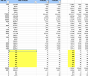
Well not sure why this isn't working. I followed your steps and the first row works but the lines below it only show the RED even if the number is greater than the forecast. I've pasted a copy below along with a screen shot of the formula. What am i doing wrong here?

QTY SOLD 12 MNTH	Feb. 23	Jan. 23	Dec. 22	Nov. 22	Oct. 22	Sept. 22	Aug. 22	Jul. 22	Jun. 22	May. 22	Apr. 22	Mar. 22	Feb. 22	Year Forecast	Forecast	Forecast	Forecast	Forecast	Forecast	Forecast	Forecast	Forecast	Forecast	Forecast	Forecast	Forecast	Forecast
189355	5000	20000	15000	25000	17500​	12500​	15000​	15000​	15000​	15000​	9355​	17500​	7500​	210,867	17484	17484	17484	17484	17484	17484	17484	17484	17484	17484	17484	17484	17484
1500	0	0	0	0	1500​	0​	0​	0​	0​	0​	0​	0​	0​	6,292	237	237	237	237	237	237	237	237	237	237	237	237	237
63000	1000	6000	7000	5000	5000​	5000​	5000​	5000​	5000​	10000​	3000​	6000​	0​	69,018	5,835	5,835	5,835	5,835	5,835	5,835	5,835	5,835	5,835	5,835	5,835	5,835	5,835
60640	0	0	16740	0	10000​	5000​	0​	6000​	4000​	10000​	4000​	4900​	0​	75,640	5,002	5,002	5,002	5,002	5,002	5,002	5,002	5,002	5,002	5,002	5,002	5,002	5,002
1000	0	0	0	0	0​	0​	0​	400​	0​	0​	0​	600​	0​	2,243	180	180	180	180	180	180	180	180	180	180	180	180	180
1252000	10000	120000	120000	60000	100000​	60000​	90000​	110000​	120000​	120000​	100000​	70000​	172000​	1,205,027	102,565	102,565	102,565	102,565	102,565	102,565	102,565	102,565	102,565	102,565	102,565	102,565	102,565
240000	0	0	30000	30000	60000​	0​	40000​	10000​	10000​	14000​	0​	16000​	30000​	168,266	7,480	7,480	7,480	7,480	7,480	7,480	7,480	7,480	7,480	7,480	7,480	7,480	7,480
1456200	800000	0	200000	50100	100000​	0​	90000​	20000​	30000​	30000​	60000​	30000​	46100​	471,931	14,184	14,184	14,184	14,184	14,184	14,184	14,184	14,184	14,184	14,184	14,184	14,184	14,184
460000	20000	31000	30000	40000	30000​	30000​	50000​	50000​	30000​	20000​	30000​	49000​	50000​	513,270	41,926	41,926	41,926	41,926	41,926	41,926	41,926	41,926	41,926	41,926	41,926	41,926	41,926
84162	1000	12000	5948	8000	12000​	4512​	2380​	4000​	8000​	4000​	11000​	4002​	7320​	82,944	7,073	7,073	7,073	7,073	7,073	7,073	7,073	7,073	7,073	7,073	7,073	7,073	7,073

 

[etaf]

you are only selecting to row 11 - which is why its just that section to J11

OCT 22 column looks like TEXT when i copied into a spreadsheet - so will not compare

you can see the numbers are right justified

Try cell * 1 = see if you get a number or a value error

where does the data come from

enter data into some cells , manually and make it so they are bigger then the forecast and it will then turn green , i'm sure

 

[DocRogers]

you are only selecting to row 11 - which is why its just that section to J11

OCT 22 column looks like TEXT when i copied into a spreadsheet - so will not compare

you can see the numbers are right justified

Try cell * 1 = see if you get a number or a value error

where does the data come from

enter data into some cells , manually and make it so they are bigger then the forecast and it will then turn green , i'm sure

I was only testing the first 11 rows so that was why it is showing that. I will cover the whole sheet once I've figured out the error. I just wanted to work with a smaller group as i thought it would be easier. I will reformat the cells to just numbers to fix the text error. I will try the Cell * 1= to see about the error. The data is generated from my ERP system as an excel file. Thank you, I will let you know what happens.

 

[etaf]

some of the values i have changed and manually entered , and the thy do turn red

Aug/Sep

you can see the zero 0 are left justified -- usually means text and where i have overwritten and manually entered have turn red

if you put the file on to a share - I can take a futher look

problem here is the XL2BB add -in reformats and shows as Rigth justified !!!!!

Book4
	A	B	C	D	E	F	G	H	I	J	K	L	M	N	O	P	Q	R	S	T	U	V	W	X	Y	Z	AA	AB
1	QTY SOLD 12 MNTH	Feb. 23	Jan. 23	Dec. 22	Nov. 22	Oct. 22	Sept. 22	Aug. 22	Jul. 22	Jun. 22	May. 22	Apr. 22	Mar. 22	Feb. 22	Year Forecast	Forecast	Forecast	Forecast	Forecast	Forecast	Forecast	Forecast	Forecast	Forecast	Forecast	Forecast	Forecast	Forecast
2	189355	5000	20000	15000	25000	17500	12500	15000	15000	15000	15000	9355	17500	7500	210,867	17484	17484	17484	17484	17484	17484	17484	17484	17484	17484	17484	17484	17484
3	1500	0	0	0	0	1500	0	0	0	0	0	0	0	0	6,292	237	237	237	237	237	237	237	237	237	237	237	237	237
4	63000	1000	6000	7000	5000	5000	5000	5000	5000	5000	10000	3000	6000	0	69,018	5,835	5,835	5,835	5,835	5,835	5,835	5,835	5,835	5,835	5,835	5,835	5,835	5,835
5	60640	0	0	16740	0	10000	5000	0	4000	4000	10000	4000	4900	0	75,640	5,002	5,002	5,002	5,002	5,002	5,002	5,002	5,002	5,002	5,002	5,002	5,002	5,002
6	1000	0	0	0	0	0	0	0	400	0	0	0	600	0	2,243	180	180	180	180	180	180	180	180	180	180	180	180	180
7	1252000	10000	120000	120000	60000	100000	60000	90000	110000	120000	120000	100000	70000	172000	1,205,027	102,565	102,565	102,565	102,565	102,565	102,565	102,565	102,565	102,565	102,565	102,565	102,565	102,565
8	240000	0	0	30000	30000	60000	0	40000	10000	10000	14000	0	16000	30000	168,266	7,480	7,480	7,480	7,480	7,480	7,480	7,480	7,480	7,480	7,480	7,480	7,480	7,480
9	1456200	800000	0	200000	50100	100000	0	90000	20000	30000	30000	60000	30000	46100	471,931	14,184	14,184	14,184	14,184	14,184	14,184	14,184	14,184	14,184	14,184	14,184	14,184	14,184
10	460000	20000	31000	30000	40000	30000	30000	50000	50000	30000	20000	30000	49000	50000	513,270	41,926	41,926	41,926	41,926	41,926	41,926	41,926	41,926	41,926	41,926	41,926	41,926	41,926
11	84162	1000	12000	5948	8000	12000	4512	2380	4000	8000	4000	11000	4002	7320	82,944	7,073	7,073	7,073	7,073	7,073	7,073	7,073	7,073	7,073	7,073	7,073	7,073	7,073
Sheet1

Cells with Conditional Formatting
Cell	Condition		Cell Format	Stop If True
A2:N11	Expression	=A2>O2	text	YES
A2:N11	Expression	=W2<O2	text	YES

I only tend to goto OneDrive, Dropbox or google docs , as I'm never certain of other random share sites and possible virus.
Please make sure you have a representative data sample and also that the data has been desensitised, remember this site is open to anyone with internet access to see - so any sensitive / personal data should be removed

Dropbox - File Deleted - Simplify your life

www.dropbox.com

 

[DocRogers]

some of the values i have changed and manually entered , and the thy do turn red

Aug/Sep

you can see the zero 0 are left justified -- usually means text and where i have overwritten and manually entered have turn red

if you put the file on to a share - I can take a futher look

problem here is the XL2BB add -in reformats and shows as Rigth justified !!!!!

Book4
	A	B	C	D	E	F	G	H	I	J	K	L	M	N	O	P	Q	R	S	T	U	V	W	X	Y	Z	AA	AB
1	QTY SOLD 12 MNTH	Feb. 23	Jan. 23	Dec. 22	Nov. 22	Oct. 22	Sept. 22	Aug. 22	Jul. 22	Jun. 22	May. 22	Apr. 22	Mar. 22	Feb. 22	Year Forecast	Forecast	Forecast	Forecast	Forecast	Forecast	Forecast	Forecast	Forecast	Forecast	Forecast	Forecast	Forecast	Forecast
2	189355	5000	20000	15000	25000	17500	12500	15000	15000	15000	15000	9355	17500	7500	210,867	17484	17484	17484	17484	17484	17484	17484	17484	17484	17484	17484	17484	17484
3	1500	0	0	0	0	1500	0	0	0	0	0	0	0	0	6,292	237	237	237	237	237	237	237	237	237	237	237	237	237
4	63000	1000	6000	7000	5000	5000	5000	5000	5000	5000	10000	3000	6000	0	69,018	5,835	5,835	5,835	5,835	5,835	5,835	5,835	5,835	5,835	5,835	5,835	5,835	5,835
5	60640	0	0	16740	0	10000	5000	0	4000	4000	10000	4000	4900	0	75,640	5,002	5,002	5,002	5,002	5,002	5,002	5,002	5,002	5,002	5,002	5,002	5,002	5,002
6	1000	0	0	0	0	0	0	0	400	0	0	0	600	0	2,243	180	180	180	180	180	180	180	180	180	180	180	180	180
7	1252000	10000	120000	120000	60000	100000	60000	90000	110000	120000	120000	100000	70000	172000	1,205,027	102,565	102,565	102,565	102,565	102,565	102,565	102,565	102,565	102,565	102,565	102,565	102,565	102,565
8	240000	0	0	30000	30000	60000	0	40000	10000	10000	14000	0	16000	30000	168,266	7,480	7,480	7,480	7,480	7,480	7,480	7,480	7,480	7,480	7,480	7,480	7,480	7,480
9	1456200	800000	0	200000	50100	100000	0	90000	20000	30000	30000	60000	30000	46100	471,931	14,184	14,184	14,184	14,184	14,184	14,184	14,184	14,184	14,184	14,184	14,184	14,184	14,184
10	460000	20000	31000	30000	40000	30000	30000	50000	50000	30000	20000	30000	49000	50000	513,270	41,926	41,926	41,926	41,926	41,926	41,926	41,926	41,926	41,926	41,926	41,926	41,926	41,926
11	84162	1000	12000	5948	8000	12000	4512	2380	4000	8000	4000	11000	4002	7320	82,944	7,073	7,073	7,073	7,073	7,073	7,073	7,073	7,073	7,073	7,073	7,073	7,073	7,073
Sheet1

Cells with Conditional Formatting
Cell	Condition		Cell Format	Stop If True
A2:N11	Expression	=A2>O2	text	YES
A2:N11	Expression	=W2<O2	text	YES

I only tend to goto OneDrive, Dropbox or google docs , as I'm never certain of other random share sites and possible virus.
Please make sure you have a representative data sample and also that the data has been desensitised, remember this site is open to anyone with internet access to see - so any sensitive / personal data should be removed

Dropbox - File Deleted - Simplify your life

www.dropbox.com

I've put a copy in dropbox WIP.xlsx

 

[DocRogers]

I've put a copy in dropbox WIP.xlsx

So I was thinking about what you said and I went through the numbers in my Forecast columns and retyped them and boom the formula worked. I tried just formatting the cells but even if I pick number it still isn't recognizing them as numbers so it looks like i will have to retype them all to make this work or at least the first column and then I can drag and copy them to the rest of the Forecast columns.

 

[etaf]

yes, the Forecast looks like text in that file

Edit
seems you have code 202 -
I used
=SUBSTITUTE(W2,CHAR(CODE(LEFT(W2))),"")*1

in a new cell and that cleared it and created a number .........

the system is generating hidden characters and so you may need to use the above formula to change to a number

other things like
text to columns
*1 +0
Copy 1 and paste special multiply did not work

if you try and Left,Right , Centre justify the number do not do that and in the formula bar you can see there are something - hidden characters -

you can see here

 

[DocRogers]

Thank you for the help. I got everything working correctly.