Conditional data validation with variable list length

[Pepess]

Hello,

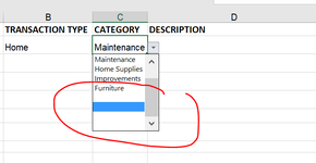
I have a conditional drop down list (column C: Category) which depends from column B: Transaction type.
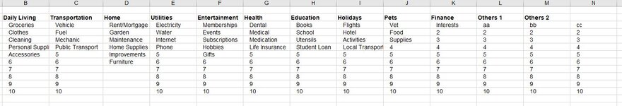
The lists for the data validation of both columns is variable, i.e. elements can be added or deleted from the list according to necessity.

For transaction type I can add up to 13 elements in my list and it works without showing up blanks in case there are less than 13 elements. Here's the formula as reference:
=OFFSET(Lists2!$B$11;0;0;1;IFERROR(MATCH("";Lists2!$B$11:$N$11;0)-1;13))

Now I need to make the category drop down list "dynamic" so that up to 10 elements can be added in the list, but if there are less, no blanks are beeing shown. I've been trying with this formula but doesn't work as I want and need some help to come further:
=OFFSET(Lists2!$B$11;1;MATCH($B2;Lists2!$B$11:$N$11;0)-1;IFERROR(MATCH("";Lists2!$B$12:$N$21;0)-1;10);1)

A screenshot of the lists for the data validation is attached.

I really appreciate your support, thanks in advance!

 

[Pepess]

I forgot to mention: all cells contain formula, since they refer from another list. Therefore, I was using the match function to find the empty cell, instead of using counta function.

 

[jaeiow]

If you set it up with a dynamic array formula that excludes blanks, you could put something like "='Lists2'!$B$12#"

 

[Pepess]

If you set it up with a dynamic array formula that excludes blanks, you could put something like "='Lists2'!$B$12#"

Hi jaeiow, thank you for your response. Would you mind to explain that a bit more? Where would you use the part you shared: "='Lists2'!$B$12#"?

 

[Fluff]

If you set it up with a dynamic array formula that excludes blanks

How? the OP is using xl2010

 

[kevin9999]

Maybe this?

=OFFSET(Lists2!$B$11,1,MATCH($B$2,Lists2!$B$11:$N$11,0)-1,SUMPRODUCT((OFFSET(Lists2!$B$11,1,MATCH($B$2,Lists2!$B$11:$N$11,0)-1,10,1)<>"")*1),1)

 

[Pepess]

Maybe this?

=OFFSET(Lists2!$B$11,1,MATCH($B$2,Lists2!$B$11:$N$11,0)-1,SUMPRODUCT((OFFSET(Lists2!$B$11,1,MATCH($B$2,Lists2!$B$11:$N$11,0)-1,10,1)<>"")*1),1)

Hi kevin, thank you! Unfortunately the formula is not working at all for me

 

[kevin9999]

Hi kevin, thank you! Unfortunately the formula is not working at all for me

I've just noticed that your regional settings use semicolons rather than commas for delimiters. Give this a try instead:

=OFFSET(Lists2!$B$11;1;MATCH($B$2;Lists2!$B$11:$N$11;0)-1;SUMPRODUCT((OFFSET(Lists2!$B$11;1;MATCH($B$2;Lists2!$B$11:$N$11,0)-1;10;1)<>"")*1);1)

 

[Pepess]

I've just noticed that your regional settings use semicolons rather than commas for delimiters. Give this a try instead:

=OFFSET(Lists2!$B$11;1;MATCH($B$2;Lists2!$B$11:$N$11;0)-1;SUMPRODUCT((OFFSET(Lists2!$B$11;1;MATCH($B$2;Lists2!$B$11:$N$11,0)-1;10;1)<>"")*1);1)

I had replaced the comas with semicolons already, but I just get #N/A

 

[kevin9999]

I had replaced the comas with semicolons already, but I just get #N/A

The #N/A error usually means that the formula can't find a referenced value. When I set up a test data set, I set the validation list for cell B2 as the range $B$11:$N$11 on the sheet called "Lists2". Is yours exactly the same? A sample of your actual data would be a big help