Conditional format based on number of days over stated date

[GJJ]

Hi all, I'm having trouble working this one out, not sure if anyone can help me out?
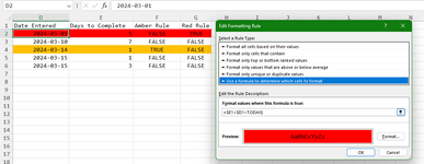
So I'm trying to stay on top of multiple ongoing tasks, and trying to colour code my tasks depending on how far past the time for an update is. For example, if I'm altering something today, I'll add todays date in cell D2, and then the number of days before I need to chase up in cell E2, which could be 1, 2, 7, 14 days etc (these would be manually entered depending on my task). So I need the formula to check against the inputted, and how many days past that date it is. If it is equal to the amount of days for me to chase, I want it turn amber, and if it is over the date, it needs to turn red.
Is this possible, or am I not going to get anywhere with this?
Thanks in advance

 

[Joe4]

Welcome to the Board!

Where are these dates that you want to compare to?
What is the address where they can be found?

 

[awoohaw]

As @Joe4 says it is unclear exactly what you want. But, this can give you a start:

Book1
	D	E	F	G
1	Date Entered	Days to Complete	Amber Rule	Red Rule
2	2024-03-01	5	FALSE	TRUE
3	2024-03-10	7	FALSE	FALSE
4	2024-03-14	1	TRUE	FALSE
5	2024-03-15	1	FALSE	FALSE
6	2024-03-15	3	FALSE	FALSE
Sheet1

Cell Formulas
Range	Formula
F2:F6	F2	=D2+E2=TODAY()
G2:G6	G2	=D2+E2<TODAY()

Cells with Conditional Formatting
Cell	Condition		Cell Format	Stop If True
E1:E6	Expression	=E1+D1<TODAY()	text	NO
E1:E6	Expression	=E1+D1=TODAY()	text	NO

 

[GJJ]

I'd manually type the date of the update Cell D2 e.g.15/3/24 then if I'd put 2 days in cell E3, on the 17/3/24 the line would turn amber, on the 18/3/24 or anytime after, the line would turn red

 

[awoohaw]

I'd manually type the date of the update Cell D2 e.g.15/3/24 then if I'd put 2 days in cell E3, on the 17/3/24 the line would turn amber, on the 18/3/24 or anytime after, the line would turn red

I'm guessing you meant E2 instead of E3. Take a look at the suggestion in Post #3.

 

[GJJ]

I'm guessing you meant E2 instead of E3. Take a look at the suggestion in Post #3.

Yes sorry, E2. Thank you, I'll take a look and see if I can get it working. Really appreciate your help

 

[awoohaw]

Yes sorry, E2. Thank you, I'll take a look and see if I can get it working. Really appreciate your help

THanks, Here is a suggestion highlighting rows:

Mr Excel Questions 75.xlsm
	D	E	F	G
1	Date Entered	Days to Complete	Amber Rule	Red Rule
2	2024-03-01	5	FALSE	TRUE
3	2024-03-10	7	FALSE	FALSE
4	2024-03-14	1	TRUE	FALSE
5	2024-03-15	1	FALSE	FALSE
6	2024-03-15	3	FALSE	FALSE
Sheet7

Cell Formulas
Range	Formula
F2:F6	F2	=D2+E2=TODAY()
G2:G6	G2	=D2+E2<TODAY()

Cells with Conditional Formatting
Cell	Condition		Cell Format	Stop If True
E1:E6,D2:D6,F2:G6	Expression	=$E1+$D1<TODAY()	text	NO
E1:E6,D2:D6,F2:G6	Expression	=$E1+$D1=TODAY()	text	NO

 

[GJJ]

THanks, Here is a suggestion highlighting rows:

Mr Excel Questions 75.xlsm
	D	E	F	G
1	Date Entered	Days to Complete	Amber Rule	Red Rule
2	2024-03-01	5	FALSE	TRUE
3	2024-03-10	7	FALSE	FALSE
4	2024-03-14	1	TRUE	FALSE
5	2024-03-15	1	FALSE	FALSE
6	2024-03-15	3	FALSE	FALSE
Sheet7

Cell Formulas
Range	Formula
F2:F6	F2	=D2+E2=TODAY()
G2:G6	G2	=D2+E2<TODAY()

Cells with Conditional Formatting
Cell	Condition		Cell Format	Stop If True
E1:E6,D2:D6,F2:G6	Expression	=$E1+$D1<TODAY()	text	NO
E1:E6,D2:D6,F2:G6	Expression	=$E1+$D1=TODAY()	text	NO

This is exactly what I'm trying to achieve, but not sure how you are doing the conditional formatting?
What type of rule do I use? How do I set it up, can't see the option to set it up with the layout you have here.

 

[awoohaw]

The "Amber" and "Red" rules are how I build the Conditional Formatting rules.
When you're satisfied with the formula for the rule(s) then you use what is in the first cell (top row) to use as the formatting rule.
Since you're asking for highlighting a ROW, the rule will be fixed for the COLUMN.
When you have the rule you like, press F2 on the top row of one rule. Copy the rule in its entirety, press [ESC] to get out of the cell.
From the home TAB, click Conditional Formatting >> NEW RULE >> Use a Formula To Set Conditional Formatting
In the following Dialog box, paste the rule into the formula entry box. If you want to highlight a row, be sure you precede the COLUMN letter with a dollar sign ($).
Click the FORMAT button.
Choose your fill or other formatting options.
Click OK or APPLY until you're out.

Repeat for the second RULE.

Then copy and paste the formatting wherever you wish.

 

[GJJ]

That has worked great, only thing that I could improve on with this really is that when no dates are entered, it is showing up as red, how would I get this to stay with no fill? So if I wanted to add lines at the bottom that were ready to be filled in, currently these are showing up as red, but ideally would want them as white until I've added the info.