Conditional Format of Row for the Next File to Open

[MrDB4Excel]

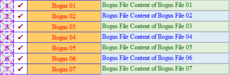
The attached XL2bb Mini Sheet shows in cell A1 the number 21 which is the next blank cell in B column.
I would like to use conditional formatting to highlight the entire row based on the cell number that appears in A1 as a visual guide to open, in this case, Bogus 20 file, to get file content to enter into, in this case, cell D21.
And I would like to do this without using any VBA. Is this possible?
Any help is much appreciated.

BogusData.xlsx
	A	B	C	D
1	21		File Name	Brief File Content
2	1	ü	Bogus 01	Bogus File Content of Bogus File 01
3	2	ü	Bogus 02	Bogus File Content of Bogus File 02
4	3	ü	Bogus 03	Bogus File Content of Bogus File 03
5	4	ü	Bogus 04	Bogus File Content of Bogus File 04
6	5	ü	Bogus 05	Bogus File Content of Bogus File 05
7	6	ü	Bogus 06	Bogus File Content of Bogus File 06
8	7	ü	Bogus 07	Bogus File Content of Bogus File 07
9	8	ü	Bogus 08	Bogus File Content of Bogus File 08
10	9	ü	Bogus 09	Bogus File Content of Bogus File 09
11	10	ü	Bogus 10	Bogus File Content of Bogus File 10
12	11	ü	Bogus 11	Bogus File Content of Bogus File 11
13	12	ü	Bogus 12	Bogus File Content of Bogus File 12
14	13	ü	Bogus 13	Bogus File Content of Bogus File 13
15	14	ü	Bogus 14	Bogus File Content of Bogus File 14
16	15	ü	Bogus 15	Bogus File Content of Bogus File 15
17	16	ü	Bogus 16	Bogus File Content of Bogus File 16
18	17	ü	Bogus 17	Bogus File Content of Bogus File 17
19	18	ü	Bogus 18	Bogus File Content of Bogus File 18
20	19	ü	Bogus 19	Bogus File Content of Bogus File 19
21	20		Bogus 20
22	21		Bogus 21
23	22		Bogus 22
24	23		Bogus 23
25	24		Bogus 24
26	25		Bogus 25
27	26		Bogus 26
Sheet1

Cell Formulas
Range	Formula
A1	A1	=MIN(IF(B2:B109="",ROW(B2:B109)))
Press CTRL+SHIFT+ENTER to enter array formulas.

 

[Fluff]

Select a2 to D109 & use this formula in CF

=ROW()=$A$1

 

[MrDB4Excel]

Easy Peasy, many thanks Fluff. Works exactly as hoped.
Happy New Year

 

[Fluff]

You're welcome & thanks for the feedback.

 

[MrDB4Excel]

How about another approach to entering the symbol in the B Column when the relevant cell in the A Column is changed to the format that tells me the file has been viewed. It is as you see, a light blue fill, bold purple text, and a red dash cross thru. In other words, for example, as soon as I mark, in this case, cell A21 that shows number 20, as viewed using the “Viewed” cell style, then cell B21 gets the checkmark thus sending the conditional formatting to the next row because cell B20 is blank.

BogusData.xlsx
	A	B	C	D
1	21		File Name	Brief File Content
2	1	ü	Bogus 01	Bogus File Content of Bogus File 01
3	2	ü	Bogus 02	Bogus File Content of Bogus File 02
4	3	ü	Bogus 03	Bogus File Content of Bogus File 03
5	4	ü	Bogus 04	Bogus File Content of Bogus File 04
6	5	ü	Bogus 05	Bogus File Content of Bogus File 05
7	6	ü	Bogus 06	Bogus File Content of Bogus File 06
8	7	ü	Bogus 07	Bogus File Content of Bogus File 07
9	8	ü	Bogus 08	Bogus File Content of Bogus File 08
10	9	ü	Bogus 09	Bogus File Content of Bogus File 09
11	10	ü	Bogus 10	Bogus File Content of Bogus File 10
12	11	ü	Bogus 11	Bogus File Content of Bogus File 11
13	12	ü	Bogus 12	Bogus File Content of Bogus File 12
14	13	ü	Bogus 13	Bogus File Content of Bogus File 13
15	14	ü	Bogus 14	Bogus File Content of Bogus File 14
16	15	ü	Bogus 15	Bogus File Content of Bogus File 15
17	16	ü	Bogus 16	Bogus File Content of Bogus File 16
18	17	ü	Bogus 17	Bogus File Content of Bogus File 17
19	18	ü	Bogus 18	Bogus File Content of Bogus File 18
20	19	ü	Bogus 19	Bogus File Content of Bogus File 19
21	20		Bogus 20
22	21		Bogus 21
23	22		Bogus 22
24	23		Bogus 23
25	24		Bogus 24
26	25		Bogus 25
27	26		Bogus 26
Sheet1

Cell Formulas
Range	Formula
A1	A1	=MIN(IF(B2:B109="",ROW(B2:B109)))
Press CTRL+SHIFT+ENTER to enter array formulas.

 

[Fluff]

Conditional formatting cannot put a value in a cell, just change the way it's displayed.

 

[MrDB4Excel]

View attachment 54228

Conditional formatting cannot put a value in a cell, just change the way it's displayed.

Okay, forget to do any conditional formatting but just be able to enter the symbol in the B Column when the relevant cell in the A Column is changed by the user via cell style to the format that tells me the file has been viewed, as seen in the attached image.
Does this make sense? What I want is not to have to manually insert the checkmark symbol each time a file is opened and viewed but that the insertion of the checkmark happens automatically when a cell in A Column has the cell style applied manually.

 

[Fluff]

No direct to way, as there is no way of knowing if the cell style has changed.

 

[MrDB4Excel]

Okay, thanks anyway.

 

[Fluff]

Glad to help & thanks for the feedback.