Conditional formatting from multiple cell data to multiple cells when data is selected from a drop down menu

grumpytrashpanda

New Member
Joined
Oct 6, 2022
Messages
8
Office Version
  1. 365
Platform
  1. Windows
Hey folks, I am okay with excel for the most part, but I am having trouble trying to define what I actually want to have happen in my spreadsheet.

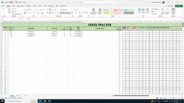
I am creating a worksheet to track book series that I have read or started reading. I've added a picture of the worksheet so you can, hopefully see what I am talking about.

As an example of what I am looking to do, in cell E4, I have 1 book read in the series. Cell F4 shows there are 8 books in the series published. And cell G4 indicates the series is completed. The G column is a drop where I can either select Completed or In Progress.

When Completed is selected, I want cell J4 to automatically fill with that purple color and cells K2 to Q8 to fill with the pink, and then the rest of the cells up to BV to be that blue color.

When In Progress is selected, I want it to do the same thing (using row 5 as an example). J5 to M5 will turn purple, cells N5 and O5 will turn pink, and the rest of the cells, up to BV, will turn blue.

When the G column (Series Status) is blank, neither Completed or In Progress yet to be selected, I want cells J# to BV# to remain unfilled.

I have tried conditional formatting a few different ways and have gotten it so that the cells I want pink will be pink, but the cells I want purple are unfilled, and all the other cells in the J to BV range are blue. And none of this is linked to the G column. And since I have no idea what I want to do is called, Google and other searches is difficult.

Any help, even if it is just pointing me somewhere else to go for answers, is greatly appreciated. Thank you!

And if this doesn't make sense, let me know and I will try to clarify.
 

Attachments

  • Series Tracker.jpg
    Series Tracker.jpg
    95.5 KB · Views: 16

Excel Facts

How to show all formulas in Excel?
Press Ctrl+` to show all formulas. Press it again to toggle back to numbers. The grave accent is often under the tilde on US keyboards.
you will need multiple rules and areas selected -

so select J2:J100 or what ever row and then use a rule
=$G2="Completed" -
Fill Purple
then select K2:Q100
=$G2="Completed"
Fill Pink
then select R2:BV100
=$G2="completed"
fill Blue

Now repeat the selections of ranges and use
=$G2="In Progress"
and fill

Book8
ABCDEFGHIJKLMNOPQRSTUV
1
2completed
3
4in progress
5completed
6completed
7in progress
8
9
10When Completed is selected, I want cell J4 to automatically fill with that purple color and cells K2 to Q8 to fill with the pink, and then the rest of the cells up to BV to be that blue color.
11
12When In Progress is selected, I want it to do the same thing (using row 5 as an example). J5 to M5 will turn purple, cells N5 and O5 will turn pink, and the rest of the cells, up to BV, will turn blue.
13
14When the G column (Series Status) is blank, neither Completed or In Progress yet to be selected, I want cells J# to BV# to remain unfilled.
15
16
Sheet1
Cells with Conditional Formatting
CellConditionCell FormatStop If True
P2:V8Expression=$G2="in progress"textNO
N2:O8Expression=$G2="in progress"textNO
J2:M8Expression=$G2="in progress"textNO
R2:V7Expression=$G2="completed"textNO
J2:J7Expression=$G2="completed"textNO
K2:Q8Expression=$G2="Completed"textNO


this will only be available on dropbox for a few days
 
Upvote 0
you will need multiple rules and areas selected -

so select J2:J100 or what ever row and then use a rule
=$G2="Completed" -
Fill Purple
then select K2:Q100
=$G2="Completed"
Fill Pink
then select R2:BV100
=$G2="completed"
fill Blue

Now repeat the selections of ranges and use
=$G2="In Progress"
and fill

Book8
ABCDEFGHIJKLMNOPQRSTUV
1
2completed
3
4in progress
5completed
6completed
7in progress
8
9
10When Completed is selected, I want cell J4 to automatically fill with that purple color and cells K2 to Q8 to fill with the pink, and then the rest of the cells up to BV to be that blue color.
11
12When In Progress is selected, I want it to do the same thing (using row 5 as an example). J5 to M5 will turn purple, cells N5 and O5 will turn pink, and the rest of the cells, up to BV, will turn blue.
13
14When the G column (Series Status) is blank, neither Completed or In Progress yet to be selected, I want cells J# to BV# to remain unfilled.
15
16
Sheet1
Cells with Conditional Formatting
CellConditionCell FormatStop If True
P2:V8Expression=$G2="in progress"textNO
N2:O8Expression=$G2="in progress"textNO
J2:M8Expression=$G2="in progress"textNO
R2:V7Expression=$G2="completed"textNO
J2:J7Expression=$G2="completed"textNO
K2:Q8Expression=$G2="Completed"textNO


this will only be available on dropbox for a few days
Thank you for your response, unfortunately, while the formulas you provided were helpful, they didn't link with the cells in columns E and F. Do you know how to integrate those as well?
 
Upvote 0
Sorry not following -
they didn't link with the cells in columns E and F. Do you know how to integrate those as well?
As an example of what I am looking to do, in cell E4, I have 1 book read in the series. Cell F4 shows there are 8 books in the series published.
And then you go on to talk about the conditions in column G showing completed and in progress and as a result of that is chosen in column G - you mentioned colours in various ranges if - G has "completed" or "in progress"

So i dont know how the conditional formatting is linked to E or F - can you expand please
Maybe give some examples - very difficult to see that image

A SMALL sample spreadsheet, around 10-20 rows, would help a lot here, with all sensitive data removed, and expected results mocked up and manually entered, with a few notes of explanation.

MrExcel has a tool called “XL2BB” that lets you post samples of your data and will allow us to copy/paste your sample data into our Excel spreadsheets, saving a lot of time.

You can also test to see if it works ok, in the "Test Here" forum.

OR if you cannot get XL2BB to work, or have restrictions on your PC , then put the sample spreadsheet onto a share
I only tend to goto OneDrive, Dropbox or google docs , as I'm never certain of other random share sites and possible virus.
Please make sure you have a representative data sample and also that the data has been desensitised, remember this site is open to anyone with internet access to see - so any sensitive / personal data should be removed
 
Upvote 0
Sorry not following -


And then you go on to talk about the conditions in column G showing completed and in progress and as a result of that is chosen in column G - you mentioned colours in various ranges if - G has "completed" or "in progress"

So i dont know how the conditional formatting is linked to E or F - can you expand please
Maybe give some examples - very difficult to see that image

A SMALL sample spreadsheet, around 10-20 rows, would help a lot here, with all sensitive data removed, and expected results mocked up and manually entered, with a few notes of explanation.

MrExcel has a tool called “XL2BB” that lets you post samples of your data and will allow us to copy/paste your sample data into our Excel spreadsheets, saving a lot of time.

You can also test to see if it works ok, in the "Test Here" forum.

OR if you cannot get XL2BB to work, or have restrictions on your PC , then put the sample spreadsheet onto a share
I only tend to goto OneDrive, Dropbox or google docs , as I'm never certain of other random share sites and possible virus.
Please make sure you have a representative data sample and also that the data has been desensitised, remember this site is open to anyone with internet access to see - so any sensitive / personal data should be removed
I am so sorry for the confusion.

2023 Read Log Work in Progress.xlsx
ABCDEFGHIJKLMNOPQRSTUVWXYZAAABAC
1SERIES #UP TO DATE?SERIES NAMEAUTHOR(S)# READ# IN SERIESSERIES STATUSFAVORITE BOOKAVE RATING= READ= TO BE READ= DOES NOT EXIST/NOT WRITTEN YET
21234567891011121314151617181920
31NoYY240
42YesXX180
530
640
750
860
970
1080
1190
12100
13110
14120
15130
Series
Cell Formulas
RangeFormula
I3:I15I3=IFERROR(AVERAGE($J3:$BV3),"0")
Cells with Conditional Formatting
CellConditionCell FormatStop If True
J3:BV502Expression=IF($G3,AND(J$2>$E3,J$2<=$F3), "Completed")textNO
Cells with Data Validation
CellAllowCriteria
B3:B15List=Categories!$Q$2:$Q$3
G3:G15List=Categories!$R$2:$R$3


As you can see, column E is the # of books read in that series and column F is the # of books in that series that has been published.

When I select either Completed or In Progress from the drop down menu in Column G, Series Status, I want the cells, starting with Column J to automatically color according the code right above it. Purple to match column E, Pink to match column F, and Blue to match the rest of the cells in the row, up to Column BV.

So using Row 4 as an example, I have read 2 (Column E) books of a 4 (Column F) book series. When I select either Completed or In Progress from Series Status (Column G), I want Cells J4:K4 to automatically highlight Purple, Cells L4:M4 to automatically color Pink, and Cells N4:BV4 to automatically color blue. I want all other cells in that grid (J5:BV503) to remain white, until either Completed or In Progress has been selected in those rows.

I hope this is clarifying!
 
Upvote 0
So using Row 4 as an example, I have read 2 (Column E) books of a 4 (Column F) book series. When I select either Completed or In Progress from Series Status (Column G), I want Cells J4:K4 to automatically highlight Purple, Cells L4:M4 to automatically color Pink, and Cells N4:BV4 to automatically color blue. I want all other cells in that grid (J5:BV503) to remain white, until either Completed or In Progress has been selected in those rows.

And column E & F are not mentioned - in the comments as to if they need to be coloured
BUT see

I'm assuming those colours in J to AC on the XL2BB
is the colour based on the number in the cells E and F

in the examples
E has 2
F has 4
So
J&K will be highlighted Purple - 2 only read , indicated by column E
L&M will be highlighted Pink - as 4 in the series in total - so 4 would be J,K,L.M and as 2 only read , indicated by column E, that leaves 2 to read in series hence L&M will be pink
Nto End - will be Blue - as the F only has 4 - so from 5to end would be blue as NONE exist in series

Next example
in the examples
E has 1
F has 8
So
only J will be highlighted Purple - 1 only read , indicated by column E
K,L,M,N,O,P,Q will be highlighted Pink - as 8 total in the series in total - so 7 not read and so would be K,L,M,N,O,P,Q and as 1 only read , indicated by column E, that leaves 7 to read in series henceK,L,M,N,O,P,Q will be pink
R to End - will be Blue - as the F only has 8 - so from 9th to end would be blue as NONE exist in series

Is that understanding correct at all ?
 
Upvote 0
so i think i have done the
INPROGRESS
But i'm not sure we need it - to be completed or inprogress - as the E & F would decide that

I'm assuming when you have completed - then there would be NO pink as none left in the series to read
and E and F would have the same number


ingnore the status - for now
is row 9
Series 7 Highligheted YELLOW
is that the conditional formatting you want
Only Purple for the 10 cells and then blue for the rest
as Read all 10 in series - so NO Pink

In which case status can be ignored - and that all the conditional formatting you need - which i can modify to ignore Status

anyway - a start

complete-inprogress-CF-ETAF.xlsx
ABCDEFGHIJKLMNOPQRSTUVWXYZAAABAC
1SERIES #UP TO DATE?SERIES NAMEAUTHOR(S)# READ# IN SERIESSERIES STATUSFAVORITE BOOKAVE RATING= READ= TO BE READ= DOES NOT EXIST/NOT WRITTEN YET
21234567891011121314151617181920
31NoYY24in progress0
42YesXX18in progress0
5344complete0
6488complete0
751012in progress0
860
971010in progress0
1080
1190
12100
13110
14120
15130
Sheet2
Cell Formulas
RangeFormula
I3:I15I3=IFERROR(AVERAGE($J3:$BV3),"0")
Cells with Conditional Formatting
CellConditionCell FormatStop If True
J3:AC15Expression=AND($G3="in Progress", J$2>$F3)textNO
J3:AC15Expression=AND($G3="in Progress", J$2<=$E3)textNO
J3:AC15Expression=AND($G3="in Progress", J$2<=$F3)textNO


Sheet2 of this file
 
Upvote 0
Solution
so i think i have done the
INPROGRESS
But i'm not sure we need it - to be completed or inprogress - as the E & F would decide that

I'm assuming when you have completed - then there would be NO pink as none left in the series to read
and E and F would have the same number


ingnore the status - for now
is row 9
Series 7 Highligheted YELLOW
is that the conditional formatting you want
Only Purple for the 10 cells and then blue for the rest
as Read all 10 in series - so NO Pink

In which case status can be ignored - and that all the conditional formatting you need - which i can modify to ignore Status

anyway - a start

complete-inprogress-CF-ETAF.xlsx
ABCDEFGHIJKLMNOPQRSTUVWXYZAAABAC
1SERIES #UP TO DATE?SERIES NAMEAUTHOR(S)# READ# IN SERIESSERIES STATUSFAVORITE BOOKAVE RATING= READ= TO BE READ= DOES NOT EXIST/NOT WRITTEN YET
21234567891011121314151617181920
31NoYY24in progress0
42YesXX18in progress0
5344complete0
6488complete0
751012in progress0
860
971010in progress0
1080
1190
12100
13110
14120
15130
Sheet2
Cell Formulas
RangeFormula
I3:I15I3=IFERROR(AVERAGE($J3:$BV3),"0")
Cells with Conditional Formatting
CellConditionCell FormatStop If True
J3:AC15Expression=AND($G3="in Progress", J$2>$F3)textNO
J3:AC15Expression=AND($G3="in Progress", J$2<=$E3)textNO
J3:AC15Expression=AND($G3="in Progress", J$2<=$F3)textNO


Sheet2 of this file
OMG! It worked, and it's beautiful. Thank you so much for your help. Now that you've shown me how it works, I'll be able to figure it out in the future. Thank you! Have a wonderful day.
 
Upvote 0
you are welcome

If you are happy to do the rest - Then i suspect you dont need the status inprogess or completed - if that row i mentioned is correct

=AND($G3="in Progress", J$2>$F3)
=AND($G3="in Progress", J$2<=$E3)
=AND($G3="in Progress", J$2<=$F3

remove the AND and Status

= J$2>$F3
=J$2<=$E3
=J$2<=$F3

is all you need

Anyway - if happy to continue alone - thats of course is fine
 
Upvote 0

Forum statistics

Threads
1,215,048
Messages
6,122,862
Members
449,097
Latest member
dbomb1414

We've detected that you are using an adblocker.

We have a great community of people providing Excel help here, but the hosting costs are enormous. You can help keep this site running by allowing ads on MrExcel.com.
Allow Ads at MrExcel

Which adblocker are you using?

Disable AdBlock

Follow these easy steps to disable AdBlock

1)Click on the icon in the browser’s toolbar.
2)Click on the icon in the browser’s toolbar.
2)Click on the "Pause on this site" option.
Go back

Disable AdBlock Plus

Follow these easy steps to disable AdBlock Plus

1)Click on the icon in the browser’s toolbar.
2)Click on the toggle to disable it for "mrexcel.com".
Go back

Disable uBlock Origin

Follow these easy steps to disable uBlock Origin

1)Click on the icon in the browser’s toolbar.
2)Click on the "Power" button.
3)Click on the "Refresh" button.
Go back

Disable uBlock

Follow these easy steps to disable uBlock

1)Click on the icon in the browser’s toolbar.
2)Click on the "Power" button.
3)Click on the "Refresh" button.
Go back
Back
Top